
Identification with confidence boxes does not care whether the frontier is convex: a certificate compares two boxes, objective by objective. This vignette runs the procedure on the frontier shapes that trouble scalarised methods (weighted sums find only the convex hull) and on near-ties, and shows what the three sets look like in each case.
make_sim <- function(means, h = 0.08) {
  function(alternative, n) {
    mu <- means |> filter(alternative == .env$alternative)
    tibble(y1 = runif(n, mu$y1 - h, mu$y1 + h),
           y2 = runif(n, mu$y2 - h, mu$y2 + h))
  }
}
run <- function(means, epsilon = 0.04, seed = 1, ...) {
  d <- pareto_design(alternatives = means$alternative, objectives = c("y1", "y2"),
                     bounds = c(0, 1), alpha = 0.05, epsilon = epsilon, max_evaluations = 4000, ...)
  set.seed(seed)
  pareto_run(d, make_sim(means), batch = 5, initial = 5)
}
Convex frontier
convex <- tribble(
  ~alternative,  ~y1,  ~y2,
  "A",          0.10, 0.80,
  "B",          0.25, 0.50,
  "C",          0.45, 0.30,
  "D",          0.80, 0.15,
  "E",          0.50, 0.60,
  "F",          0.70, 0.45
)
s <- run(convex)
plausible_pareto_set(s)
#>
#> ── Pareto sets ──
#>
#> • Estimated frontier: "A", "B", "C", and "D"
#> • Plausible: "A", "B", "C", and "D"
#> • Certified optimal: A, B, C, D
#> • Uncertain: none
#> • Certified dominated: E, F
#> ✔ Identified: every alternative is certified.
autoplot(s)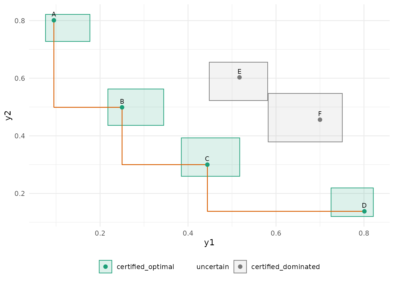
Concave (non-convex) frontier
The middle alternative C is Pareto-optimal but lies
above the segment that joins its neighbours, so no weighted sum of the
objectives would select it. The boxes certify it without difficulty.
concave <- tribble(
  ~alternative,  ~y1,  ~y2,
  "A",          0.10, 0.80,
  "B",          0.30, 0.65,
  "C",          0.45, 0.55,
  "D",          0.60, 0.30,
  "E",          0.80, 0.10,
  "F",          0.55, 0.70
)
s <- run(concave)
plausible_pareto_set(s)$table |>
  select(alternative, status, dominated_by, n_evaluations)
#> # A tibble: 6 × 4
#>   alternative status              dominated_by n_evaluations
#>   <chr>       <chr>               <chr>                <int>
#> 1 A           certified_optimal   NA                      90
#> 2 B           certified_optimal   NA                     315
#> 3 C           certified_optimal   NA                     215
#> 4 D           certified_optimal   NA                      80
#> 5 E           certified_optimal   NA                      90
#> 6 F           certified_dominated C                       90
autoplot(s)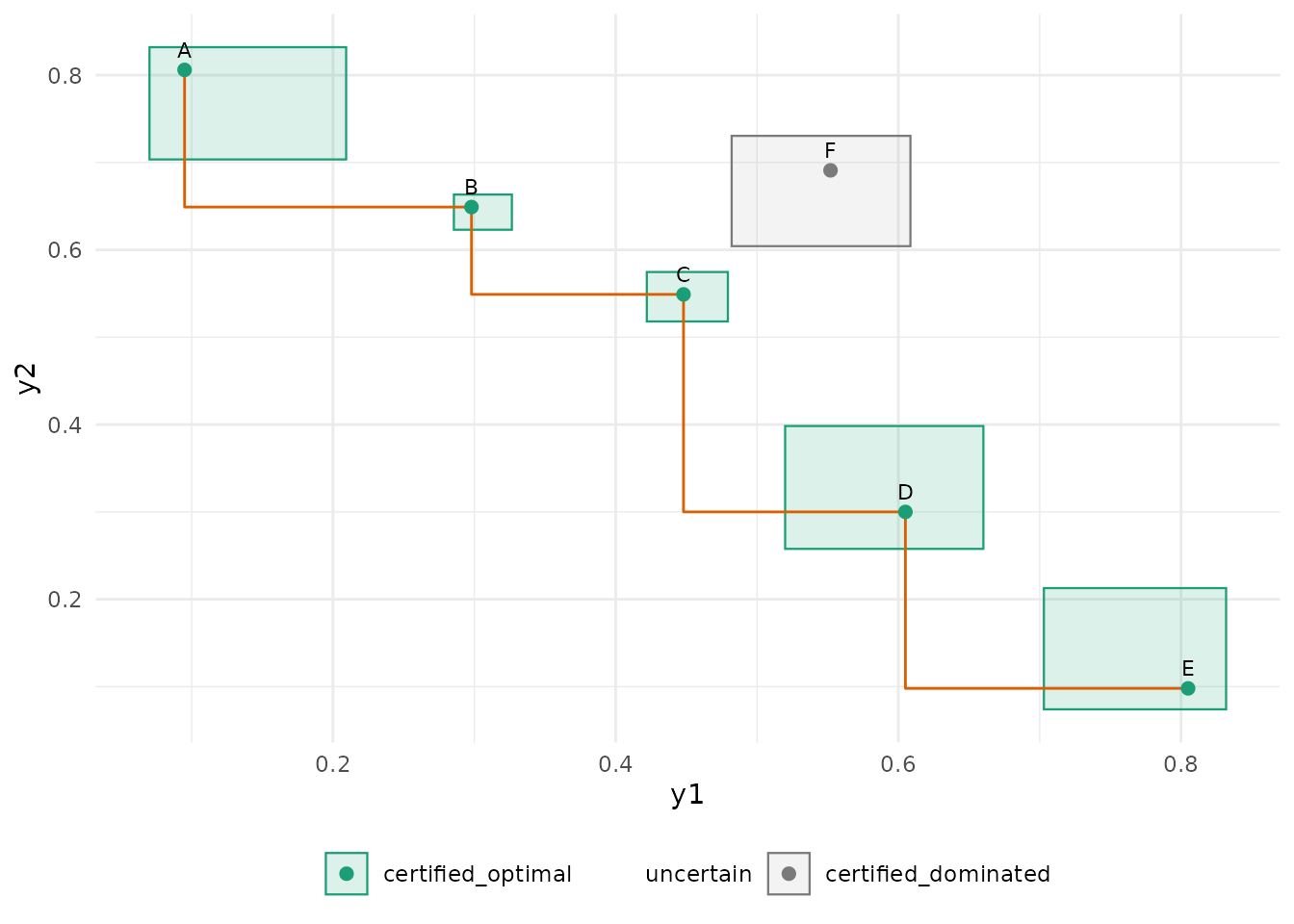
Disconnected frontier
Two clusters of optimal alternatives with a dominated gap between them.
disconnected <- tribble(
  ~alternative,  ~y1,  ~y2,
  "A",          0.10, 0.85,
  "B",          0.15, 0.75,
  "C",          0.70, 0.20,
  "D",          0.80, 0.12,
  "E",          0.45, 0.55,
  "F",          0.40, 0.65
)
s <- run(disconnected)
plausible_pareto_set(s)$table |>
  select(alternative, status, dominated_by, n_evaluations)
#> # A tibble: 6 × 4
#>   alternative status            dominated_by n_evaluations
#>   <chr>       <chr>             <chr>                <int>
#> 1 A           uncertain         NA                    1635
#> 2 B           certified_optimal NA                     205
#> 3 C           certified_optimal NA                     210
#> 4 D           certified_optimal NA                     440
#> 5 E           certified_optimal NA                     215
#> 6 F           uncertain         NA                    1295
autoplot(s)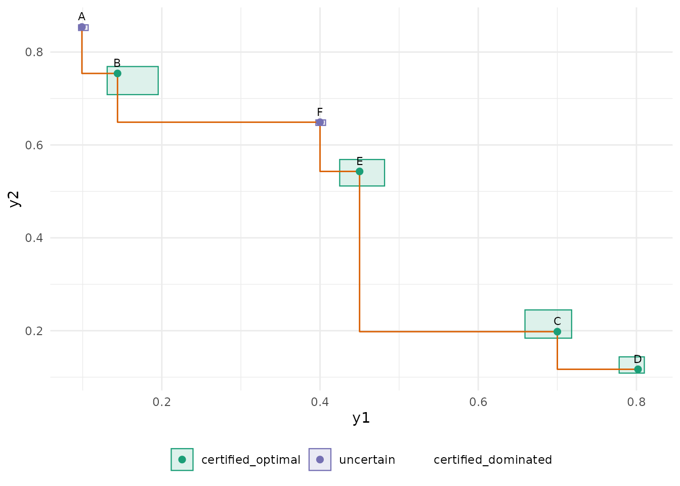
Near-ties
Two alternatives within 0.02 of each other on both objectives, with a
tolerance of 0.04: they are an epsilon-tie. The procedure
keeps the first in design order as the representative and certifies the
other as dominated by it; the report names the tie. With a tolerance
below the gap the two could not be separated and the identification
would run to its budget.
ties <- tribble(
  ~alternative,  ~y1,  ~y2,
  "A",          0.20, 0.60,
  "B",          0.21, 0.61,
  "C",          0.60, 0.20,
  "D",          0.50, 0.50
)
s <- run(ties, epsilon = 0.04)
plausible_pareto_set(s)$table |>
  select(alternative, status, dominated_by, n_evaluations)
#> # A tibble: 4 × 4
#>   alternative status              dominated_by n_evaluations
#>   <chr>       <chr>               <chr>                <int>
#> 1 A           certified_optimal   NA                     280
#> 2 B           certified_dominated A                      280
#> 3 C           certified_optimal   NA                      50
#> 4 D           uncertain           NA                    3390
s_tight <- run(ties, epsilon = 0.005)
glance(s_tight) |>
  select(n_evaluations, n_uncertain, stopping_reason)
#> # A tibble: 1 × 3
#>   n_evaluations n_uncertain stopping_reason
#>           <int>       <int> <chr>
#> 1          4000           1 max_evaluations
Reading the plots
In every plot the boxes are the simultaneous confidence boxes, the
colour is the status, and the orange step line joins the point estimates
of the estimated frontier. A box that overlaps the region to the lower
left of another box’s corner cannot be certified dominated; a box
entirely to the upper right of another one’s upper-right corner (shifted
by epsilon) is.