Validation

A sampling package must earn trust the design-based way: the inclusion probabilities it claims must be the ones it delivers. This vignette checks the package’s promises by simulation — every number below is recomputed when the vignette is built.

library(chromy)
set.seed(20261022)

The sample size is always exact

Not on average: always. Ten thousand selections, every one with exactly the expected hits it was asked for.

frame <- data.frame(size = rlnorm(150, 2))
n_hits <- replicate(10000, {
  s <- chromy_sample(frame, n = 23, size = "size")
  sum(s$sample$hits)
})
table(n_hits)
#> n_hits
#>    23 
#> 10000

Expected hits are delivered

For each unit, the fraction of selections in which it was hit must converge to its expected hits. The largest absolute deviation over the whole frame, against the Monte Carlo error it should sit within:

lambda <- expected_hits(frame$size, 23)
hits <- matrix(0L, 4000, nrow(frame))
for (r in seq_len(nrow(hits))) {
  s <- chromy_sample(frame, n = 23, size = "size")
  hits[r, s$sample$unit] <- s$sample$hits
}
observed <- colMeans(hits)
mc_se <- sqrt(lambda * (1 - lambda) / nrow(hits))

max(abs(observed - lambda))
#> [1] 0.01554681
max(abs(observed - lambda) / pmax(mc_se, 1e-6))   # in Monte Carlo SEs
#> [1] 2.430212

plot(lambda, observed,
  xlab = "expected hits", ylab = "observed frequency",
  pch = 16, col = "#35508C88", cex = 0.7
)
abline(0, 1, col = "#D9962E", lwd = 1.5)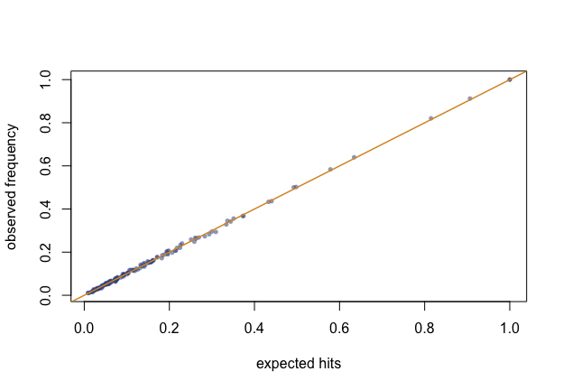

Figure of the chunk unbiased-plot

Minimum replacement holds

Hits never stray further than one from the expectation, including for units expected more than once:

heavy <- data.frame(size = c(900, 500, rlnorm(60, 2)))
ok <- replicate(2000, {
  s <- chromy_sample(heavy, n = 12, size = "size",
                     min_replacement = TRUE)
  all(s$sample$hits == floor(s$sample$expected_hits) |
      s$sample$hits == ceiling(s$sample$expected_hits))
})
all(ok)
#> [1] TRUE

The estimator is unbiased and the variance honest

The multiplicity estimator must centre on the true total; the successive-difference variance has no unbiasedness to promise under a systematic-like design, but it should sit near the Monte Carlo variance — and err on the conservative side when the serpentine order carries real structure.

pop <- data.frame(
  stratum = rep(sprintf("s%02d", 1:10), each = 30),
  size    = rlnorm(300, 2)
)
pop$y <- 50 + 10 * pop$size + rnorm(300, sd = 15)
truth <- sum(pop$y)

runs <- t(replicate(2000, {
  s <- chromy_sample(pop, n = 50, size = "size",
                     order_by = c("stratum", "chromy_size"))
  e <- estimate_total(s, "y")
  c(total = e$total, var = e$se^2)
}))

c(
  relative_bias   = mean(runs[, "total"]) / truth - 1,
  empirical_var   = var(runs[, "total"]),
  mean_sd_var     = mean(runs[, "var"]),
  variance_ratio  = mean(runs[, "var"]) / var(runs[, "total"])
)
#>  relative_bias  empirical_var    mean_sd_var variance_ratio 
#>   5.229982e-04   2.682902e+06   4.660619e+06   1.737156e+00

A ratio near one says the successive-difference variance is a fair report; above one, a conservative one.

The reference implementation

The package was distilled from a reference R implementation, kept verbatim in the test suite (tests/testthat/helper-reference.R) as an oracle: given the same seed, chromy_sample() must reproduce it draw for draw — the same head, the same uniforms, the same hits — across size-column, multivariate, serpentine, nested, residual-head and minimum-replacement designs. The Rust engine is itself pinned to the same reference by golden fixtures (tests/golden.rs in chromy-core), with the integer outputs exact and the floating-point outputs at machine precision. That check has been run against SAS itself: the validation/sas folder of the repository holds a frame of 60 units run through PROC SURVEYSELECT METHOD=PPS_SEQ (SAS 9.4, 2000 seeds) and through this package. The expected hits agree to export precision (SAS’s PPS_SEQ is pure minimum replacement, min_replacement = TRUE here; certainty resolution is SAS’s separate CERTSIZE= option), the serpentine order agrees position for position, every SAS run has the exact sample size within the minimum-replacement bounds, and the observed hit frequencies sit within Monte Carlo error of the expected hits — five checks of five. A Stata user can run the same comparison against ppschromy; the designs agree in distribution, though not draw for draw, since each system consumes its own generator.