A survey that goes to the field has two costs that textbooks keep
apart: the statistical cost, the variance of the estimator for a given
sample size, and the field cost, the travel between units and the
interviews, which is what the budget actually pays for.
fieldopt puts the two side by side. This vignette walks
through one design from the frame to the cost-variance frontier.
A frame with a depot
The frame is a data frame with one row per sampling unit (a segment, a farm, a census block) and its coordinates. One row is the depot, the office the teams leave from and return to. Here the frame is synthetic: forty segments in a 10 x 10 km square, with a crop area that trends from west to east.
library(fieldopt)
library(dplyr, warn.conflicts = FALSE)
set.seed(2026)
frame <- tibble(
  unit = c("depot", paste0("s", 1:40)),
  x = c(5, runif(40, 0, 10)), y = c(5, runif(40, 0, 10))
) |>
  mutate(crop = if_else(unit == "depot", NA_real_, 20 + 3 * x + rnorm(n(), sd = 2)))
frame
#> # A tibble: 41 × 4
#>    unit      x     y  crop
#>    <chr> <dbl> <dbl> <dbl>
#>  1 depot 5     5      NA
#>  2 s1    6.99  3.71   42.5
#>  3 s2    5.57  8.75   34.3
#>  4 s3    1.40  4.35   24.8
#>  5 s4    2.86  4.40   26.9
#>  6 s5    5.55  0.820  39.5
#>  7 s6    0.251 0.346  22.2
#>  8 s7    4.66  9.29   33.2
#>  9 s8    8.61  2.95   47.4
#> 10 s9    2.53  5.19   28.4
#> # ℹ 31 more rows
A real frame usually starts as a spatial object:
as_frame() turns an sf layer of segments or
points into this data frame (centroids in latitude and longitude, the
area of each polygon), and as_sf() puts samples and results
back on the geometries for maps.
Travel and cost
travel_matrix() computes the matrix of travel distances
between all units (or, given a sample and the depot as
bases, only between the depot and the sampled units, which
is what the routing needs). With longitude and latitude it uses
great-circle distances in kilometres; with planar coordinates, as here,
Euclidean distances. A matrix computed on a road network (for example
with OSRM) can be passed through the matrix argument and is
the better input when it exists.
m <- travel_matrix(frame, method = "euclidean")
m
#> Travel matrix: 41 units, euclidean (distance); mean off-diagonal 4.886.
field_cost_model() turns a routing solution into money:
a cost per unit of travel, a fixed cost per visited unit (access,
setting up) and a cost per interview.
model <- field_cost_model(
  per_travel = 2, per_unit = 30, per_interview = 10,
  interviews_per_unit = 4, currency = "BRL"
)
model
#> Field cost model (BRL): 2 per travel unit, 0 per route, 30 per visited unit, 10
#> per interview.
Select, route, estimate
select_units() draws a spatially balanced probability
sample with the local pivotal method: the inclusion probabilities are
known, and units close to each other are rarely selected together.
Spatial balance usually lowers the variance of totals of spatially
structured variables; it also spreads the units over the territory,
which is exactly what makes the field work longer. Making that tension
explicit is the point of the package.
s <- frame |>
  filter(unit != "depot") |>
  select_units(n = 12)
s |>
  sampled() |>
  select(unit, x, y, pi)
#> # A tibble: 12 × 4
#>    unit       x     y    pi
#>    <chr>  <dbl> <dbl> <dbl>
#>  1 s3    1.40   4.35    0.3
#>  2 s6    0.251  0.346   0.3
#>  3 s8    8.61   2.95    0.3
#>  4 s11   0.0593 9.72    0.3
#>  5 s12   6.92   6.33    0.3
#>  6 s15   1.54   5.23    0.3
#>  7 s21   3.42   2.98    0.3
#>  8 s22   3.43   8.96    0.3
#>  9 s27   4.11   6.30    0.3
#> 10 s35   5.86   1.86    0.3
#> 11 s36   4.26   6.33    0.3
#> 12 s40   4.47   9.00    0.3
route_fieldwork() routes the field work from the depot
through the selected units. Without limits it returns one tour; with a
maximum length or a maximum number of stops per route, it splits the
work into routes, one per team or per day. Small instances are solved
exactly; larger ones by a hybrid genetic search with an optimal split of
the tour and a local search, with a lower bound and, for single tours, a
proof of optimality, so that the quality of the solution is visible. The
sample can be piped straight into the routing.
r <- s |>
  travel_matrix(bases = frame |> filter(unit == "depot"), method = "euclidean") |>
  route_fieldwork(units = s, depot = "depot", max_stops = 5, cost_model = model)
r
#>
#> ── Field routes ────────────────────────────────────────────────────────────────
#> 3 routes from "depot" through 12 units: total travel 42.62 distance (proven
#> optimal).
#> Route 1 (17.81): s3 > s15 > s11 > s22 > s40
#> Route 2 (21.56): s21 > s6 > s35 > s8 > s12
#> Route 3 (3.254): s36 > s27
#> Cost (BRL): travel 85.24 + routes 0 + units 360 + interviews 480 = 925.2.
autoplot(r)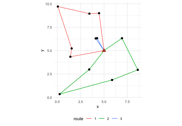
design_variance() gives the Horvitz-Thompson estimate of
the total of crop and its variance by the local-mean
estimator of Grafström and Schelin (2014), which suits spatially
balanced samples and needs no joint inclusion probabilities. The
variance the same sample size would give under simple random sampling is
shown for comparison.
design_variance(s, y = "crop")
#> # A tibble: 1 × 9
#>   total variance    se     cv variance_srs     n     N variance_method    df
#>   <dbl>    <dbl> <dbl>  <dbl>        <dbl> <int> <int> <chr>           <int>
#> 1 1254.    3158.  56.2 0.0448        5874.    12    40 local-mean         11
sum(frame$crop, na.rm = TRUE)
#> [1] 1241.484
The cost-variance frontier
A design is chosen by its sample size, its routing limits and its
cost model. cost_variance_frontier() repeats the
select-route-price-estimate cycle for a grid of sample sizes and returns
the mean cost and the mean variance at each size: the frontier a survey
planner faces.
f <- cost_variance_frontier(
  frame,
  depot = "depot", cost_model = model,
  n_grid = c(6, 9, 12, 16, 20, 24), y = "crop",
  method = "euclidean", max_stops = 5,
  n_rep = 8, iterations = 60
)
f
#> # A tibble: 6 × 9
#>       n cost_mean cost_sd cost_per_unit travel_mean routes_mean variance_mean
#> * <dbl>     <dbl>   <dbl>         <dbl>       <dbl>       <dbl>         <dbl>
#> 1     6      475.   6.08           79.2        27.6           2        13594.
#> 2     9      701.   4.64           77.9        35.5           2         4791.
#> 3    12      925.   8.47           77.1        42.7           3         2958.
#> 4    16     1218.   6.22           76.1        48.9           4         1529.
#> 5    20     1517.   0.949          75.9        58.7           4         1136.
#> 6    24     1810.   3.69           75.4        65.1           5          825.
#> # ℹ 2 more variables: cv_mean <dbl>, n_rep <dbl>
autoplot(f)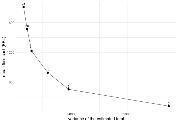
The frontier makes two questions answerable with numbers: how much
the next unit of precision costs in the field, and how much a different
field organisation (more teams, longer days, a closer depot) would
change that price. The vignettes routing-teams and
frames-and-allocation take those questions up.
References
Cochran, W. G. (1977). Sampling Techniques, third edition. Wiley.
Grafström, A., Lundström, N. L. P. and Schelin, L. (2012). Spatially balanced sampling through the pivotal method. Biometrics, 68(2), 514–520.
Grafström, A. and Schelin, L. (2014). How to select representative samples. Scandinavian Journal of Statistics, 41(2), 277–290.
Prins, C. (2004). A simple and effective evolutionary algorithm for the vehicle routing problem. Computers & Operations Research, 31(12), 1985–2002.