Validation and benchmarks • fieldopt

This vignette records how the package was checked: the routing solver against public benchmark instances and other solvers, and the estimators by simulation. The large runs were done once, outside the package build, with the scripts of the fieldopt-core repository; the small ones run here.

The routing solver

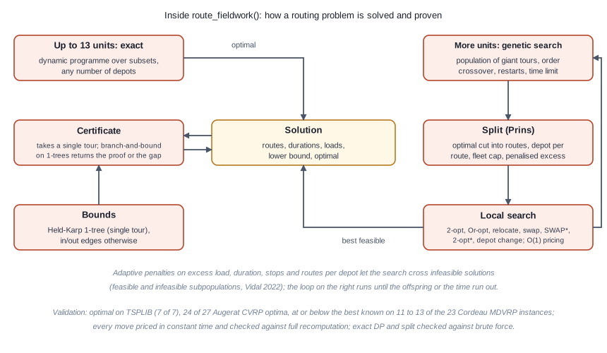
Figure of the chunk unnamed-chunk-2

Instances with rounded Euclidean distances, as the libraries define them, one core of a laptop, one seed; “proven” means the certificate closed the gap within ten seconds:

Set	Instances	Setting	Optimal	Mean gap	Largest gap	Time
TSPLIB (51 to 101 nodes)	7	2000 offspring	7 of 7 (6 proven)	0.00%	0.00%	0.7 to 4.7 s
Augerat A (CVRP, 31 to 79 customers)	27	200 offspring (default)	14 of 27	0.20%	1.14%	under 0.4 s
Augerat A	27	2000 offspring	24 of 27	0.01%	0.15%	0.7 to 4 s
Cordeau MDVRP (50 to 360 customers, 2 to 6 depots)	23	2000 offspring	11 of 23 at or below best known	0.29%	1.5%	1 to 26 s
Cordeau MDVRP	23	20 s each	13 of 23 at or below best known	0.26%	1.9%	20 s

Other solvers on the same instances: PyVRP through the vrpr package reaches 18 of 27 Augerat optima in one second and 24 in five (mean gap 0.05%); HiGHS on the compact MTZ formulation solves the TSP up to 51 nodes (21 s) but stays 40 to 60 percent away from the optimum after three minutes on the smallest Augerat instances, which is why the package does not route with a general MIP solver.

Stability: across eight seeds on four instances the gap moved by less than one percentage point (standard deviation below 0.3 points).

Internal checks in the engine’s test suite: every local-search move is priced in constant time and was checked against a full recomputation on tens of thousands of accepted moves; the exact dynamic programme and the split of giant tours were checked against brute force on hundreds of random instances with one to three depots and asymmetric costs; the lower bounds never exceed the exact optimum; an independent review found and fixed four defects before release.

The estimators

Small Monte Carlo checks, run here, of the unbiasedness of the main estimators.

set.seed(4)
cells <- expand_grid(x = 1:15, y = 1:15) |> mutate(unit = paste0("c", row_number()))
areas <- expand_grid(unit = cells$unit, k = 1:3) |>
  transmute(unit, establishment = paste0(unit, "-", k), area = 0.3, y = rlnorm(n(), 2, 0.5))
deff <- point_design_effect(
  cells, areas,
  n = 25, points_per_cell = 6, cell_size = 1, n_sim = 60, seed = 2
)
deff |> select(bias, variance, mean_variance_estimate, deff)
#> # A tibble: 1 × 4
#>     bias variance mean_variance_estimate   deff
#>    <dbl>    <dbl>                  <dbl>  <dbl>
#> 1 56.127  158401.                167223. 1.4716

set.seed(7)
cells <- cells |>
  mutate(
    domain = if_else(runif(n()) < 0.2, "ab", "a"),
    yv = if_else(domain == "ab", 80, 10) + rnorm(n(), sd = 3)
  )
overlap <- cells |> filter(domain == "ab")
lst <- bind_rows(
  overlap |> transmute(unit = paste0("l", row_number()), domain, yv),
  tibble(unit = paste0("b", 1:12), domain = "b", yv = 120 + rnorm(12, sd = 5))
) |>
  mutate(x = runif(n()), y = runif(n()))
truth <- sum(cells$yv) + sum(lst$yv[lst$domain == "b"])
est <- map(1:40, \(k) {
  sa <- cells |> select_units(n = 30, seed = k)
  sb <- lst |> select_units(n = 15, method = "srs", seed = k)
  tibble(
    hartley = dual_frame_estimator(sa, sb, "yv", "domain")$total,
    fb = dual_frame_estimator(sa, sb, "yv", "domain", estimator = "fuller-burmeister")$total
  )
}) |> list_rbind()
est |>
  summarise(across(everything(), mean)) |>
  mutate(truth = truth, .before = 1)
#> # A tibble: 1 × 3
#>    truth hartley     fb
#>    <dbl>   <dbl>  <dbl>
#> 1 6182.1  6221.3 6247.1
# relative bias in percent
est |> summarise(across(everything(), \(e) round(100 * (mean(e) - truth) / truth, 2)))
#> # A tibble: 1 × 2
#>   hartley    fb
#>     <dbl> <dbl>
#> 1    0.63  1.05

Further checks live in the test suite: the Hartley allocation against a grid search over the mixing weight, Cochran’s two-stage optimum against enumeration, the multivariate allocation against an integer grid, the cube method’s balance against simple random sampling, and the survey designs produced by as_svydesign() against the package’s own totals and replicate variances.