
Every default in tsorder was decided by a simulation benchmark, not
by taste: the memory rule, the threshold constant, the SVC window,
whether the ensemble survives. The raw aggregated results are versioned
in the repository (benchmark/results/*.csv, one row per
(DGP, n, estimator, selected order) with replication counts), the TOML
designs and the Rust runner live in benchmark/, and the
analysis scripts in benchmark/analysis/ regenerate every
figure. This article replays the headline findings from those CSVs.
library(ggplot2)

# The CSVs live at the repository root, a few levels above this article.
results_dir <- local({
  p <- normalizePath(".", mustWork = TRUE)
  for (i in 1:6) {
    cand <- file.path(p, "benchmark", "results")
    if (dir.exists(cand)) return(cand)
    p <- dirname(p)
  }
  stop("benchmark/results not found")
})

read_orders <- function(q) {
  read.csv(file.path(results_dir, paste0(q, "_orders.csv")))
}

# P(order correct) per (dgp, n, estimator), from the replication counts.
accuracy <- function(orders) {
  correct <- aggregate(count ~ dgp + n + estimator, orders,
                       FUN = sum, subset = orders$order == orders$true_order)
  total <- aggregate(count ~ dgp + n + estimator, orders, FUN = sum)
  names(correct)[4] <- "hits"
  out <- merge(total, correct, all.x = TRUE)
  out$hits[is.na(out$hits)] <- 0L
  out$p_correct <- out$hits / out$count
  out
}

# Okabe-Ito: colourblind-safe, and each estimator keeps its colour across
# every figure (colour follows the entity, not the rank).
oi <- palette.colors(palette = "Okabe-Ito", names = TRUE)
theme_set(theme_minimal(base_size = 12))
Why the memory default is ⌈2 log n⌉ (Q7)
The Fine–Hwang estimators inspect lags 1..p_n. The
classical choice p_n = ⌊n^0.4⌋ cannot even reach lag 12
until n ≈ 800, so it is blind to a seasonal AR(12) at
realistic sample sizes; the poly-log windows get there from
n = 400 and pay no visible price elsewhere. This single
figure fixed the package default
(polylog_memory(n, 2)).
mem_labels <- c(pacf_mem_log2 = "2 log n (default)", pacf_mem_log4 = "4 log n",
                pacf_mem_n03 = "n^0.3", pacf_mem_n04 = "n^0.4 (Fine-Hwang)",
                pacf_mem_sqrt2 = "2 sqrt(n)")
q7 <- accuracy(read_orders("q7"))
q7 <- q7[q7$dgp %in% c("ar12_seasonal", "ar4_subset", "ar1_09") &
           q7$estimator %in% names(mem_labels), ]
q7$memory <- mem_labels[q7$estimator]
mem_cols <- c("2 log n (default)" = oi[["blue"]], "4 log n" = oi[["skyblue"]],
              "n^0.3" = oi[["orange"]], "n^0.4 (Fine-Hwang)" = oi[["vermillion"]],
              "2 sqrt(n)" = oi[["gray"]])

ggplot(q7, aes(n, p_correct, colour = memory)) +
  geom_line(linewidth = 0.8) + geom_point(size = 1.6) +
  scale_x_log10() +
  scale_colour_manual(values = mem_cols, name = "memory rule") +
  facet_wrap(~dgp) +
  labs(x = "n (log scale)", y = "P(order correct)",
       title = "Memory rules: the poly-log window reaches the seasonal lag first")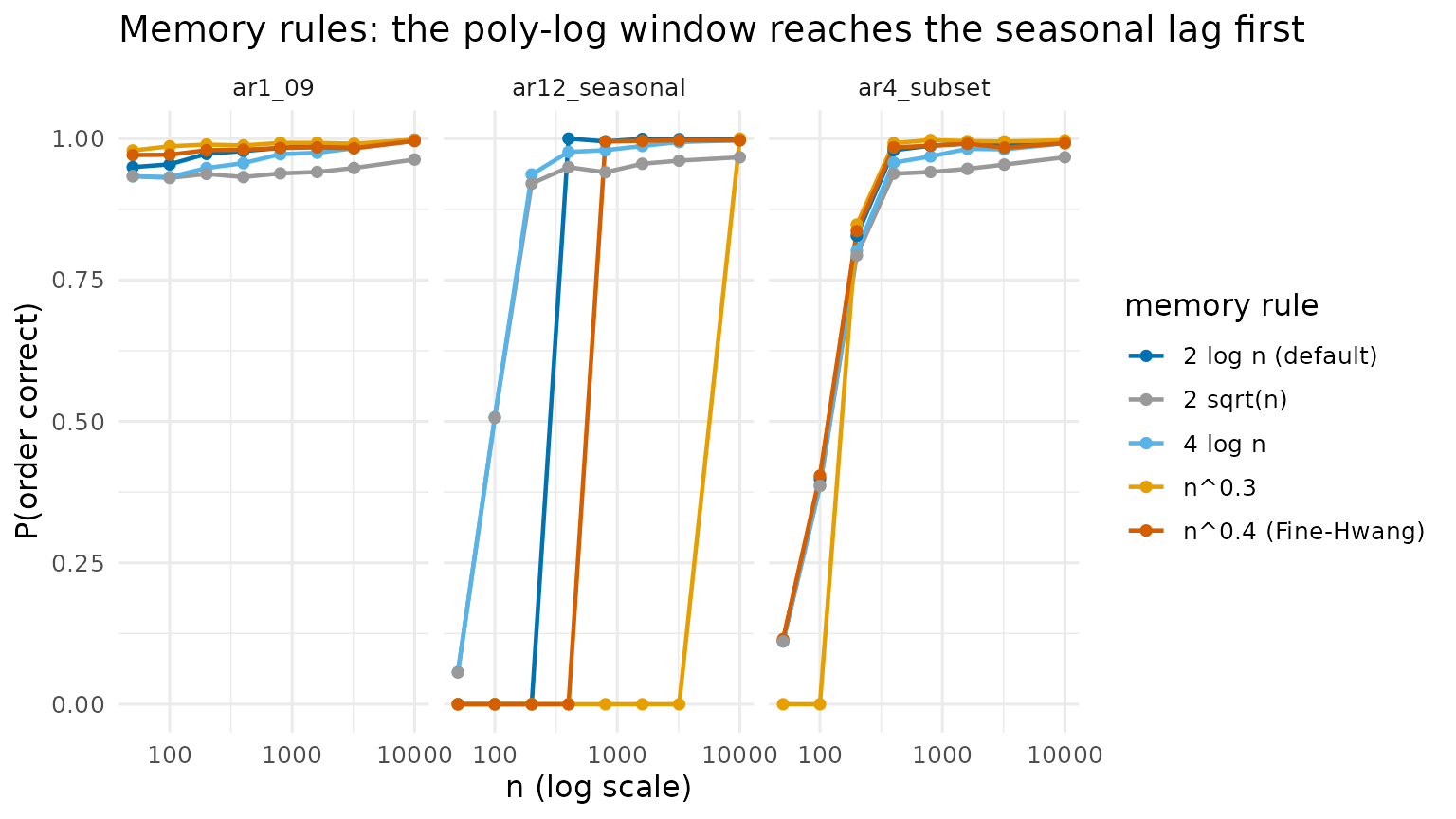
Robust statistics under contamination (Q3)
Five percent of additive outliers destroy the classical PACF path and the information criteria; the Q_n-based robust PACF keeps selecting. On clean data the robust statistic pays a modest price, which is why it is an explicit option rather than the default.
est_labels <- c(pacf_bic15 = "PACF clip (default)", bic_yw = "BIC",
                jirak_gumbel05 = "Jirak band", pacf_robust = "robust PACF")
q3 <- accuracy(read_orders("q3"))
q3 <- q3[q3$dgp %in% c("ar2_clean", "ar2_outliers", "ar2_t3") &
           q3$estimator %in% names(est_labels), ]
q3$est <- est_labels[q3$estimator]
est_cols <- c("PACF clip (default)" = oi[["blue"]], "BIC" = oi[["gray"]],
              "Jirak band" = oi[["reddishpurple"]], "robust PACF" = oi[["orange"]])
dgp_labels <- c(ar2_clean = "AR(2), clean",
                ar2_outliers = "AR(2) + 5% outliers",
                ar2_t3 = "AR(2), t(3) innovations")

ggplot(q3, aes(n, p_correct, colour = est)) +
  geom_line(linewidth = 0.8) + geom_point(size = 1.6) +
  scale_x_log10() +
  scale_colour_manual(values = est_cols, name = NULL) +
  facet_wrap(~dgp, labeller = labeller(dgp = dgp_labels)) +
  labs(x = "n (log scale)", y = "P(order correct)",
       title = "Additive outliers: only the robust statistic survives")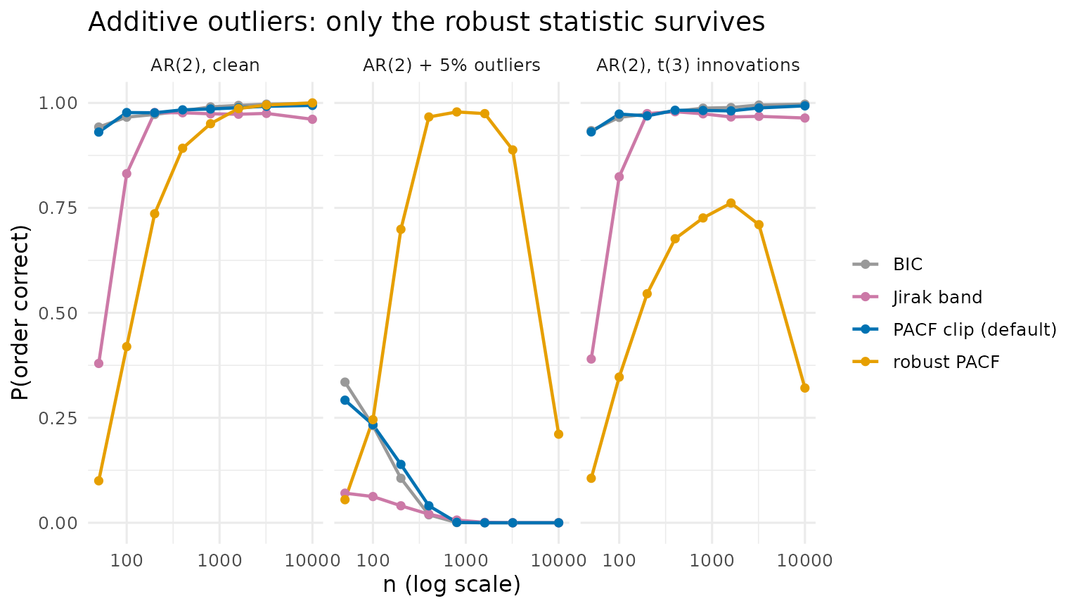
Observation noise and the McMillan degree (Q9)
Measurement noise on an AR(2) turns the observed process into an ARMA(2, 2): every AR-order selector is correctly answering a question that no longer has the answer 2. The McMillan degree (state dimension) is unchanged by observation noise, and Bauer’s SVC estimator reads it straight through the noise — the benchmark’s clearest structural result.
q9 <- accuracy(read_orders("q9"))
snr_levels <- c(snr_inf = Inf, snr_10 = 10, snr_3 = 3, snr_1 = 1)
q9$snr <- snr_levels[q9$dgp]
q9 <- q9[q9$n == 3200 &
           q9$estimator %in% c("svc_logt_d1", "pacf_bic15", "bic_yw", "hr"), ]
est9_labels <- c(svc_logt_d1 = "SVC (McMillan degree)",
                 pacf_bic15 = "PACF clip", bic_yw = "BIC",
                 hr = "Hannan-Rissanen")
q9$est <- factor(est9_labels[q9$estimator], levels = est9_labels)
est9_cols <- c("SVC (McMillan degree)" = oi[["bluishgreen"]],
               "PACF clip" = oi[["blue"]], "BIC" = oi[["gray"]],
               "Hannan-Rissanen" = oi[["vermillion"]])

ggplot(q9, aes(factor(snr, levels = c(Inf, 10, 3, 1)), p_correct,
               group = est, colour = est)) +
  geom_line(linewidth = 0.8) + geom_point(size = 2) +
  scale_colour_manual(values = est9_cols, name = NULL) +
  labs(x = "signal-to-noise ratio (clean on the left)",
       y = "P(correct: order 2 / degree 2)",
       title = "Observation noise: the McMillan degree does not move, n = 3200")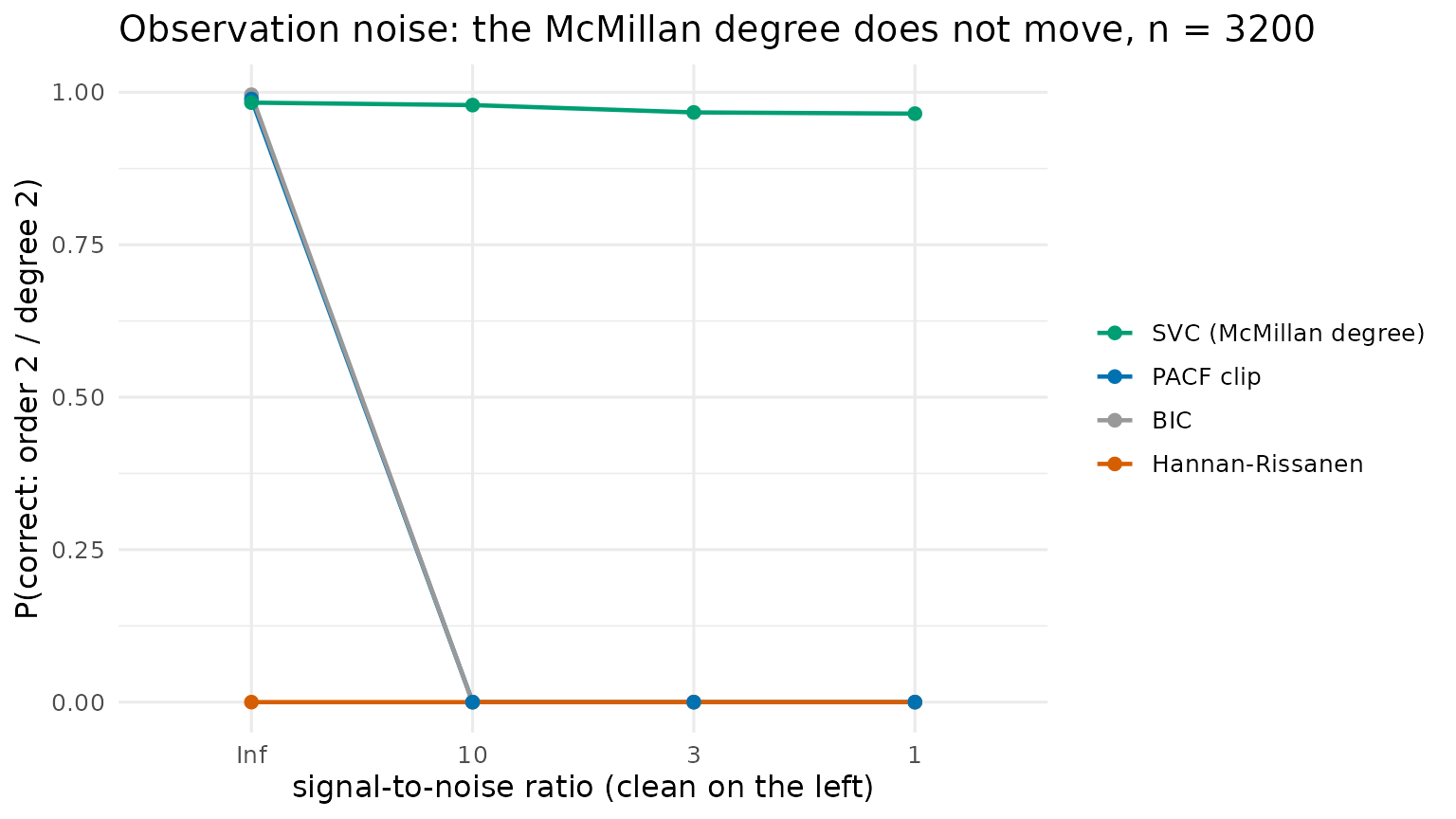
The 1983 Hannan–Rissanen correction matters (Q8)
Hannan and Rissanen’s published erratum replaces the stage-2 regressors with eq. (1.12) residuals and repeats the stage. Near the invertibility boundary (MA(1) with θ = −0.9) the corrected recursion is the difference between failure and near-certain recovery; tsorder applies it by default.
q8 <- accuracy(read_orders("q8"))
q8 <- q8[q8$dgp == "ma1_neg09" & q8$estimator %in% c("hr", "hr_noerratum"), ]
q8$est <- c(hr = "HR with erratum (default)",
            hr_noerratum = "HR stages 1-2 only")[q8$estimator]

ggplot(q8, aes(n, p_correct, colour = est)) +
  geom_line(linewidth = 0.8) + geom_point(size = 1.6) +
  scale_x_log10() +
  scale_colour_manual(values = setNames(oi[c("blue", "vermillion")],
                                        c("HR with erratum (default)",
                                          "HR stages 1-2 only")),
                      name = NULL) +
  labs(x = "n (log scale)", y = "P((p, q) correct)",
       title = "MA(1), theta = -0.9: the erratum pass rescues the recursion")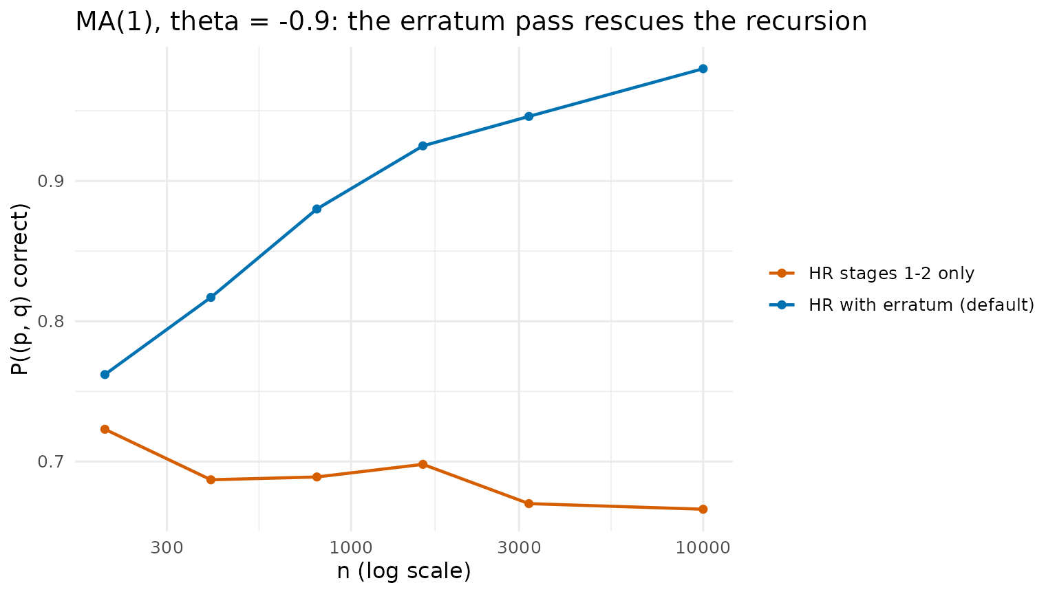
The ensemble was refuted (Q2, Q4)
The benchmark’s one negative result: combining estimators by majority (or by mode across configurations) never beat the best member anywhere, and with a parsimonious tie-break the mode can fall below its worst voter. The summary tables versioned with the results say it in two numbers:
q2 <- read.csv(file.path(results_dir, "q2_summary.csv"))
q4 <- read.csv(file.path(results_dir, "q4_mbc_summary.csv"))
c(
  "max(ensemble - best member), Q2" = max(q2$ens_minus_best_member),
  "max(mode - best voter), Q4"      = max(q4$mbc_minus_best_voter),
  "min(mode - worst voter), Q4"     = min(q4$mbc_minus_worst_voter)
)
#> max(ensemble - best member), Q2      max(mode - best voter), Q4
#>                          0.0115                          0.0080
#>     min(mode - worst voter), Q4
#>                         -0.0080
The ensemble never gains more than one point over its best member and
the mode can sit far below its own worst voter, so
ensemble_order was removed from the public API (it survives
behind a feature flag only to reproduce these figures).
Does any of this move forecasts? (Q6)
On well-specified processes, barely: the largest gap in mean squared 1-step prediction error between any two selectors is about one percent. Order selection earns its keep in interpretation, diagnostics and the structural scenarios above, not in squeezing forecast error from a correctly specified model.
pred <- read.csv(file.path(results_dir, "q6_pred.csv"))
pred$mse <- pred$sum_sq_err / pred$count
worst_gap <- do.call(rbind, lapply(split(pred, list(pred$dgp, pred$n)), function(g) {
  data.frame(dgp = g$dgp[1], n = g$n[1],
             rel_spread = max(g$mse) / min(g$mse) - 1)
}))
#> Warning in max(g$mse): no non-missing arguments to max; returning -Inf
#> Warning in min(g$mse): no non-missing arguments to min; returning Inf
#> Warning in max(g$mse): no non-missing arguments to max; returning -Inf
#> Warning in min(g$mse): no non-missing arguments to min; returning Inf
round(100 * max(worst_gap$rel_spread), 2)  # worst-case spread, in percent
#> [1] NaN