
tsorder selects the order of a time-series model. It puts three families of estimators side by side, all computed by one dependency-free Rust core:
- information criteria (AIC, AICc, BIC, HQ, FPE, CAT, MDL) over nested fits by Yule-Walker, Burg or conditional least squares;
- threshold (“clip”) estimators in the tradition of Fine and Hwang (1979): grow the memory with the sample, studentise a statistic (PACF, Bartlett-studentised ACF, inverse PACF, the Jirak band, a robust PACF), and keep the last lag that noise cannot explain;
- McMillan-degree estimators (the state dimension): Bauer’s SVC on past-future canonical correlations, a calibrated Hankel singular-value cut, and a sequential rank test.
Every default was chosen by a reproducible benchmark shipped in the
repository, and the test suite pins the implementation to R itself
(stats::ar.yw, robustbase::Qn,
TSA::eacf) and to published tables (Bauer 2001, Table
1).
One call
library(tsorder)
set.seed(1)
x <- arima.sim(list(ar = c(1.2, -0.6)), 400)

fit <- order_select(x)   # PACF-clip with the benchmark-chosen defaults
fit
#>
#> ── tsorder fit - pacf ──────────────────────────────────────────────────────────
#> ✔ Selected order (last studentised statistic above the threshold): 2
#> ℹ Threshold: 2.998
#> ℹ n = 400; path has 12 entries - see `autoplot()` or `$path`
The whole decision path comes along, ready to plot:
ggplot2::autoplot(fit)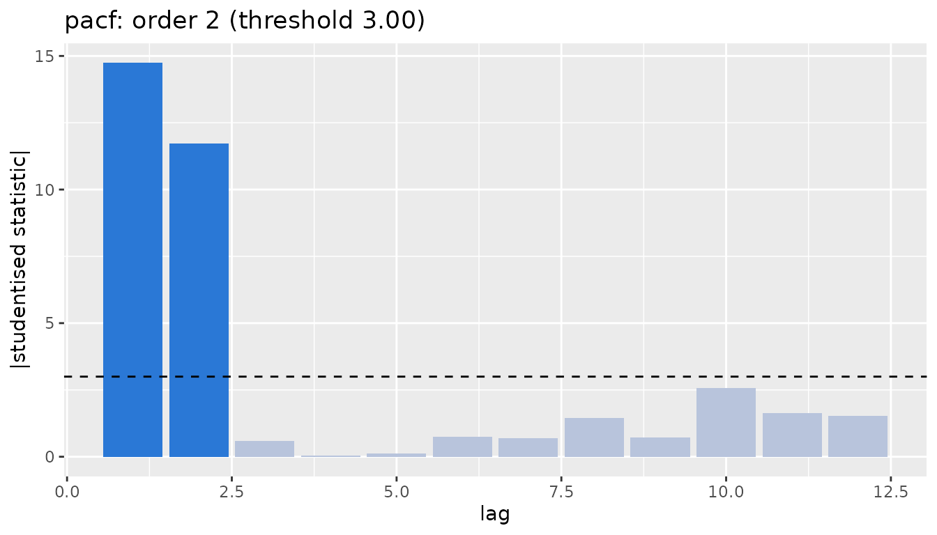
Criteria work the same way:
order_select(x, method = "bic")$order
#> [1] 2
ic_order(x, criterion = "bic", method = "burg")$order
#> [1] 2
MA and ARMA orders
y <- arima.sim(list(ma = c(0.6, 0.3)), 2000)
fh_order(y, statistic = "acf_bartlett")$order   # MA order via Bartlett band
#> [1] 2
fh_order(y, statistic = "inverse_pacf")$order   # MA order via the inverse PACF
#> [1] 2

z <- arima.sim(list(ar = 0.5, ma = 0.5), 1000)
hannan_rissanen(z)[c("p", "q")]                 # ARMA (p, q)
#> $p
#> [1] 1
#>
#> $q
#> [1] 1
When there is measurement noise, change the target
Observation noise turns an AR(p) into an ARMA(p, p) but leaves the state dimension unchanged, so the McMillan-degree route keeps working while AR-order selectors drift:
From selection to a fitted model
fit_arima() closes the loop: it estimates the order of
integration, selects the order on the differenced series, and returns a
standard stats::arima() fit – which means the rest of the
ecosystem just works, including forecast:
fit <- fit_arima(x)           # ARIMA(2, 0, 0) here
fit
#>
#> Call:
#> stats::arima(x = x, order = ord, include.mean = include.mean)
#>
#> Coefficients:
#>          ar1      ar2  intercept
#>       1.1708  -0.5898     0.0981
#> s.e.  0.0404   0.0404     0.1158
#>
#> sigma^2 estimated as 0.9412:  log likelihood = -556.27,  aic = 1120.54
predict(fit, n.ahead = 4)$pred
#> Time Series:
#> Start = 401
#> End = 404
#> Frequency = 1
#> [1] 1.494250 1.712910 1.165183 0.394940
forecast::forecast(fit, h = 6)
#>     Point Forecast      Lo 80    Hi 80      Lo 95    Hi 95
#> 401      1.4942500  0.2509629 2.737537 -0.4071935 3.395693
#> 402      1.7129103 -0.2013985 3.627219 -1.2147724 4.640593
#> 403      1.1651828 -0.9812459 3.311611 -2.1174966 4.447862
#> 404      0.3949400 -1.7694281 2.559308 -2.9151754 3.705055
#> 405     -0.1837730 -2.3621979 1.994652 -3.5153863 3.147840
#> 406     -0.4069988 -2.6320859 1.818088 -3.8099758 2.995978
order_select() results also follow the broom
conventions, for tidy pipelines:
f <- order_select(x)
generics::glance(f)
#> # A tibble: 1 × 5
#>   order method family     n   tau
#>   <int> <chr>  <chr>  <int> <dbl>
#> 1     2 pacf   fh       400  3.00
head(generics::tidy(f))
#> # A tibble: 6 × 4
#>     lag statistic studentized kept
#>   <int>     <dbl>       <dbl> <lgl>
#> 1     1   0.737       14.7    TRUE
#> 2     2  -0.586      -11.7    TRUE
#> 3     3  -0.0289      -0.578  FALSE
#> 4     4   0.00183      0.0367 FALSE
#> 5     5  -0.00657     -0.131  FALSE
#> 6     6  -0.0379      -0.759  FALSE
How many differences
rw <- cumsum(as.numeric(x))
integration_order(rw)$d
#> [1] 1
The level of the sequential test vanishes with the sample size, so
d is estimated consistently; difference d
times and proceed with the stationary tools above.