
tsorder answers one question — how many terms does this series need? — with three families of estimators that answer it in different senses. This article walks through all of them on simulated data where the truth is known. The design principle shared by everything in the package: every threshold lives on a studentised scale (each statistic is divided by its own null standard error), so “above the threshold” means the same thing for every statistic, every process and every scale.
Information criteria: penalised fit
The classical answer. Fit AR(0..K), charge each order a penalty, keep the argmin. All seven criteria (AIC, AICc, BIC, HQ, FPE, CAT, MDL) share one Levinson recursion, so asking for all of them costs one pass.
x <- as.numeric(arima.sim(list(ar = c(1.2, -0.6)), 800))
fit <- order_select(x, "bic")
fit
#>
#> ── tsorder fit - bic ───────────────────────────────────────────────────────────
#> ✔ Selected order (argmin of the criterion): 2
#> ℹ n = 800; path has 30 entries - see `autoplot()` or `$path`
autoplot(fit)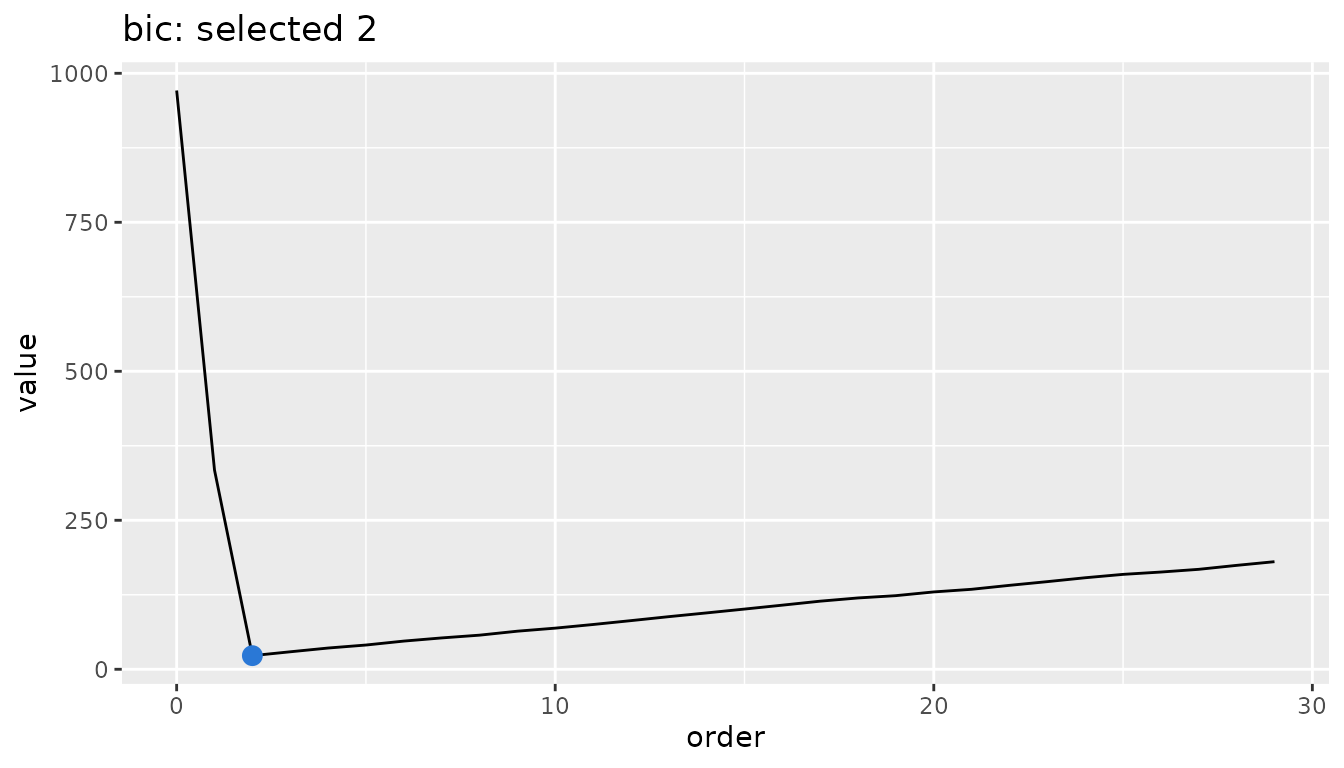
Threshold (“clip”) estimators: the last lag noise cannot explain
The Fine–Hwang (1979) family: let the inspected memory
p_n grow with the sample (default ⌈2 log n⌉),
studentise a statistic lag by lag, zero out everything below a
slowly-growing threshold, and report the last survivor. The default
statistic is the PACF, which is self-studentised: beyond the
true order its fluctuation is 1/√n whatever the process
(Quenouille).
fit <- order_select(x, "pacf")
fit
#>
#> ── tsorder fit - pacf ──────────────────────────────────────────────────────────
#> ✔ Selected order (last studentised statistic above the threshold): 2
#> ℹ Threshold: 3.167
#> ℹ n = 800; path has 14 entries - see `autoplot()` or `$path`
autoplot(fit)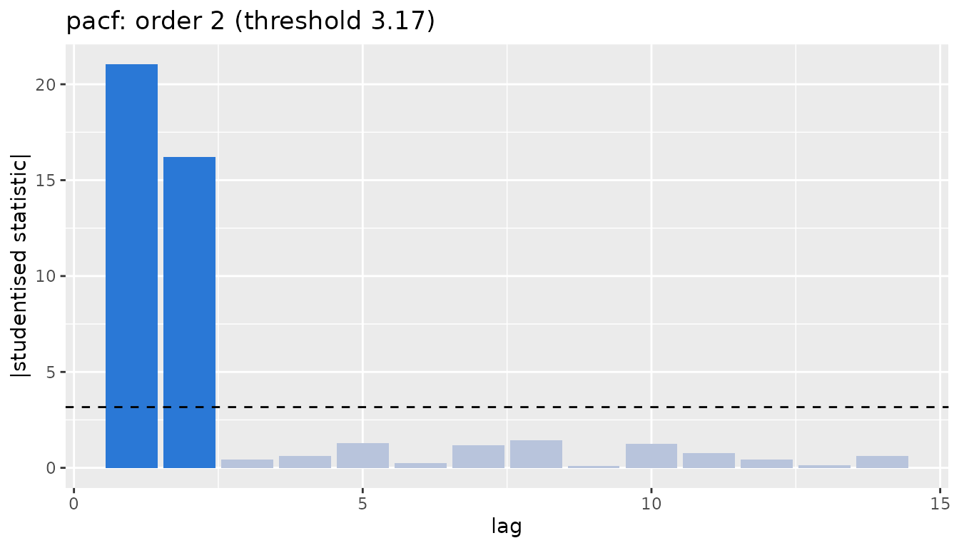
Each statistic targets a family: pacf,
jirak and long_ar_ols read AR orders;
acf_bartlett and inverse_pacf read MA
orders.
y <- as.numeric(arima.sim(list(ma = c(0.9, 0.5)), 800))
c(ma_by_acf  = order_select(y, "acf_bartlett")$order,
  ma_by_ipacf = order_select(y, "inverse_pacf")$order,
  ar_bic_overshoots = ic_order(y, "bic")$order)  # an MA is an AR(Inf)
#>         ma_by_acf       ma_by_ipacf ar_bic_overshoots
#>                 2                 2                 6
The last line is the point of having both families: an MA(2) is an AR(∞), so an AR criterion dutifully reports a long autoregression, while the MA-targeted statistics read 2.
Jirak’s refitted estimator
jirak_order() refits the Yule–Walker autoregression at
every dimension k ≤ p_n, studentises each coefficient
vector exactly, and takes the largest per-dimension estimate — extra
power when a coefficient is small in the long-AR representation, at
O(p_n⁴) cost (negligible at the poly-log default).
jirak_order(x)$order
#> [1] 2
order_select(x, "jirak_refit")
#>
#> ── tsorder fit - jirak_refit ───────────────────────────────────────────────────
#> ✔ Selected order (max over the per-dimension refits): 2
#> ℹ Threshold: 3.009
#> ℹ n = 800; path has 14 entries - see `autoplot()` or `$path`
Robust statistics for contaminated series
Five percent of additive outliers is enough to erase the classical
PACF. The robust statistics (pacf_robust,
acf_robust) replace the sample autocorrelation with the
Ma–Genton Q_n-ratio form, whose shared denominator cancels the outlier
bias. They are marked experimental: their studentisations are Monte
Carlo-calibrated, pending exact theory.
clean <- as.numeric(arima.sim(list(ar = c(1.2, -0.6)), 2000))
spikes <- rbinom(2000, 1, 0.05) * rnorm(2000, sd = 10)
dirty <- clean + spikes

c(classical_clean = order_select(clean, "pacf")$order,
  classical_dirty = order_select(dirty, "pacf")$order,
  robust_dirty    = order_select(dirty, "pacf_robust")$order)
#> classical_clean classical_dirty    robust_dirty
#>               2               4               2
McMillan degree: an order that survives measurement noise
Adding observation noise to an AR(2) makes the observed series an
ARMA(2, 2) — every AR-order selector then has a different true
answer. The McMillan degree (the state dimension, max(p, q)
for an ARMA) does not move. svc is Bauer’s (2001)
canonical-correlation estimator of it.
ar2 <- as.numeric(arima.sim(list(ar = c(1.2, -0.6)), 3000))
noisy <- ar2 + rnorm(3000, sd = 0.5 * sd(ar2))

c(svc_clean = order_select(ar2, "svc")$order,
  svc_noisy = order_select(noisy, "svc")$order,   # still the degree
  pacf_noisy = order_select(noisy, "pacf")$order) # answers a different question
#>  svc_clean  svc_noisy pacf_noisy
#>          2          2          4
ARMA (p, q) jointly
Two identifiers: the EACF table of Tsay and Tiao (vertex read automatically), and Hannan–Rissanen (with the published 1983 correction pass, on by default — see the benchmark article for why it matters).
z <- as.numeric(arima.sim(list(ar = 0.7, ma = 0.4), 1500))
eacf(z)$order
#> NULL
hannan_rissanen(z)[c("p", "q")]
#> $p
#> [1] 1
#>
#> $q
#> [1] 1
From selection to a fitted model
integration_order() estimates d by
sequential KPSS testing with a vanishing level; fit_arima()
chains everything and returns a plain stats::arima fit, so
predict(), forecast::forecast() and broom all
apply.
w <- cumsum(z)  # integrate once
integration_order(w)$d
#> [1] 1
fit <- fit_arima(w, method = "hr")
fit
#>
#> Call:
#> stats::arima(x = x, order = ord, include.mean = include.mean)
#>
#> Coefficients:
#>          ar1     ma1
#>       0.6910  0.3705
#> s.e.  0.0219  0.0278
#>
#> sigma^2 estimated as 0.9872:  log likelihood = -2117.99,  aic = 4241.99
In a tidyverts pipeline, the same chain is available as a
fabletools model:
Choosing among them
- Stationary, clean, AR-like: the default
order_select(x)(PACF clip) oric_order(x, "bic")— they agree far more often than not. - MA order:
acf_bartlettorinverse_pacf. -
pandqtogether:hannan_rissanen, oreacfto see the table. - Outliers or heavy tails:
pacf_robust/acf_robust. - Measurement noise, or you need the state dimension:
svc. - Unsure about stationarity:
integration_order()first, or letfit_arima()handle the whole chain.
The defaults behind each of these choices were fixed by the simulation benchmark described in the benchmark article.