Robustness and honest limits: recovery, distributions, and degeneracy • lcdaGRASP

The paper evaluates LCDA-GRASP/GR on five well-behaved benchmark networks. One should not conclude only from where there is data: those five networks have strong, clean community structure, and modularity is only an approximation of “good partition”. This article stresses the method along three axes that the headline tables do not show, and reports what it finds without embellishment.

The thread running through all three is a single discipline: do not trust the mean alone. Recovery degrades as communities dissolve; the per-replicate spread is wide where tables print only a point estimate; and several distinct “near-best” partitions coexist, so the one you report is somewhat arbitrary. The honest reading of the package is that LCDA-GRASP/GR is a competitive, not leading community detector, and its leader designation is valuable as a joint, community-grounded output rather than as a superior raw spreader.

1. Recovery across community-strength regimes

We sweep the mixing parameter $\mu \in [0.1, 0.8]$ on canonical LFR networks (Lancichinetti–Fortunato–Radicchi 2008) — from strong community structure ( $\mu \to 0$ ) into the regime where the planted communities dissolve — and measure $Q$ , the adjusted Rand index (ARI) and normalized mutual information (NMI) against the planted partition. $Q$ alone cannot tell you whether the recovered partition is correct; ARI/NMI can.

Generated. 2026-06-01, lcdaGRASP 0.3.1, 10 reps, n=500.

Generator: canonical LFR (Lancichinetti-Fortunato-Radicchi 2008) via networkx 3.6.1 (.venv-lfr); tau1=2.5, tau2=1.5, avg_degree=12, comm in [20,60]
n=500 fixed; size effects not explored here (see large-scale item 1.4).
IC simulator is pure R (item 2.9 = Rcpp kernel); MC and reps kept modest for runtime.
Leader-utility uses top-degree as the centrality comparator (strongest single baseline in 1.9).

library(ggplot2); library(dplyr)
#> 
#> Attaching package: 'dplyr'
#> The following objects are masked from 'package:stats':
#> 
#>     filter, lag
#> The following objects are masked from 'package:base':
#> 
#>     intersect, setdiff, setequal, union
quality <- d_lfr$results$quality
sm <- quality |>
  dplyr::group_by(mu, method) |>
  # Dispersion first: inside summarise() a later expression sees the column it
  # has just created, so sd(NMI) after NMI = mean(NMI) would receive a scalar
  # and return NA (silently dropping the ribbon below).
  dplyr::summarise(NMI_sd = sd(NMI), NMI = mean(NMI), ARI = mean(ARI),
                   Q = mean(Q), .groups = "drop")

ggplot(sm, aes(mu, NMI, colour = method, fill = method)) +
  geom_ribbon(aes(ymin = NMI - NMI_sd, ymax = NMI + NMI_sd), alpha = 0.12, colour = NA) +
  geom_line(linewidth = 0.9) + geom_point(size = 1.3) +
  labs(title = "Recovery of the planted partition (NMI vs ground truth)",
       subtitle = "Canonical LFR; shaded band = ±1 sd over replicates; higher is better",
       x = expression(mu~"(mixing parameter)"), y = "NMI") +
  theme_minimal(base_size = 10)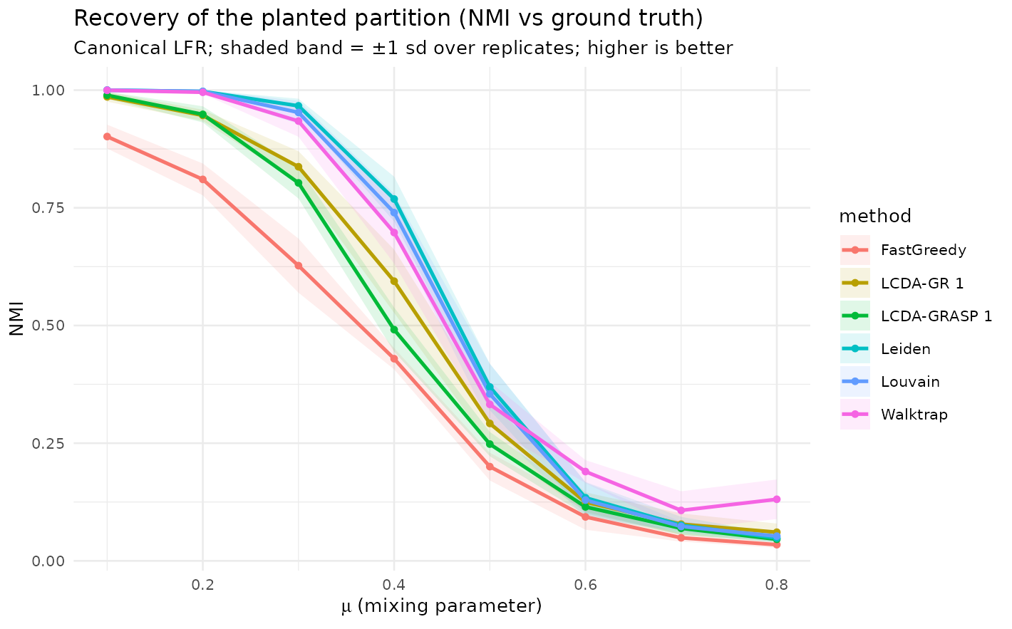

sm |>
  dplyr::filter(mu %in% c(0.2, 0.4, 0.6)) |>
  dplyr::transmute(mu, method, NMI = round(NMI, 3)) |>
  tidyr::pivot_wider(names_from = mu, values_from = NMI) |>
  knitr::kable(caption = "NMI vs the planted partition at low/medium/high mixing.")

NMI vs the planted partition at low/medium/high mixing.
method	0.2	0.4	0.6
FastGreedy	0.810	0.429	0.093
LCDA-GR 1	0.946	0.594	0.125
LCDA-GRASP 1	0.948	0.491	0.115
Leiden	0.997	0.769	0.134
Louvain	0.997	0.740	0.129
Walktrap	0.995	0.697	0.190

On canonical LFR the proposed methods recover well at low mixing but trail Leiden/Louvain — and especially ECG (ensemble clustering, Poulin & Théberge 2019), the strongest recovery baseline — across the sweep. The shaded band already makes the discipline concrete: the per-replicate sd is non-trivial, so two methods whose means cross may be indistinguishable at a given $\mu$ . The ensemble-consensus variant lcda_ecg() closes the recovery gap (see Reproducing the paper’s benchmark numbers and the lcda_ecg documentation).

Leader utility across community strength

The same pool lets us ask whether the LCDA leaders are useful seeds: we compare the expected Independent-Cascade spread from the detected leaders against an equal-size top-degree seed set, as a function of $\mu$ .

u <- d_lfr$results$leader_utility |>
  dplyr::group_by(mu) |>
  # Standard error first (see the note above: a self-referencing summarise()
  # would hand sd() the mean it has just computed and yield NA).
  dplyr::summarise(se = sd(adv_vs_degree) / sqrt(dplyr::n()),
                   adv_vs_degree = mean(adv_vs_degree),
                   adv_vs_random = mean(adv_vs_random), .groups = "drop")
ggplot(u, aes(mu, adv_vs_degree)) +
  geom_hline(yintercept = 0, linetype = 2, colour = "grey50") +
  geom_ribbon(aes(ymin = adv_vs_degree - se, ymax = adv_vs_degree + se), alpha = 0.15) +
  geom_line(linewidth = 0.9) + geom_point(size = 1.3) +
  labs(title = "Leader spreading advantage vs a top-degree seed set",
       subtitle = "Above zero: LCDA leaders out-spread top-degree of the same size",
       x = expression(mu), y = "IC-spread advantage (LCDA − top-degree)") +
  theme_minimal(base_size = 10)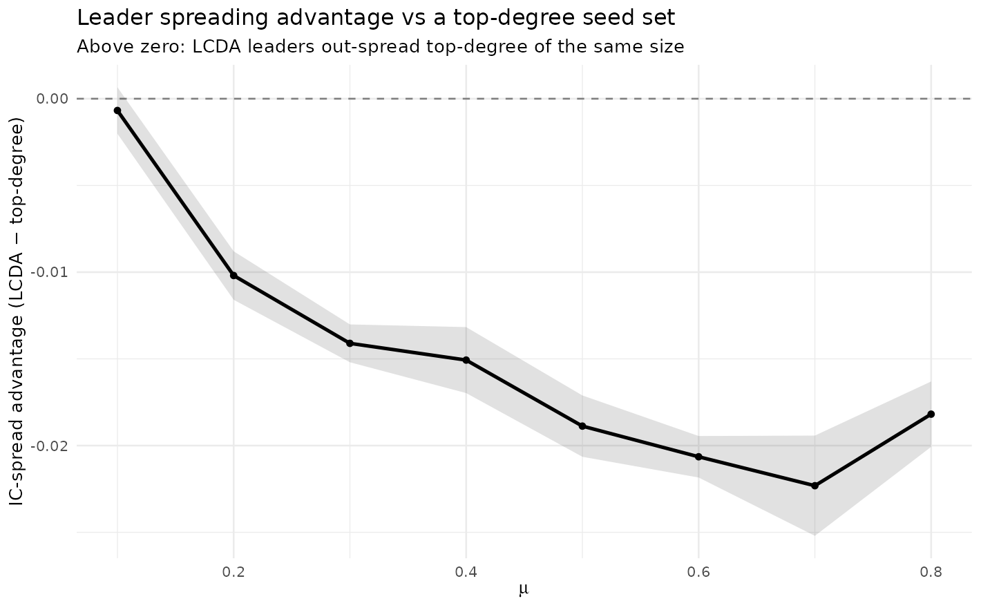

The leaders always beat a random seed set, but they do not out-spread a top-degree set on LFR. The $\pm 1$ standard-error band makes the reading precise: at the strongest-community regime the difference is indistinguishable from zero (the band still covers the dashed line), and it turns clearly negative as $\mu$ grows. The leader contribution is the joint, community-grounded designation — not superior raw spreading.

2. Distributions of Q and H, not just means

Where the paper reports means and significance letters, here we draw the boxplots, ECDFs and (Q, H) scatter that those tables hide, over replications per (graph $\times$ algorithm $\times$ centrality $\times$ similarity).

res <- d_eda$results |> dplyr::mutate(config = paste(centrality, similarity, sep = "/"))

# Q on x directly (coord_flip would silently disable the facet free scale).
ggplot(res, aes(Q, config, fill = algorithm)) +
  geom_boxplot(outlier.size = 0.5, alpha = 0.65, orientation = "y") +
  facet_wrap(~ graph, scales = "free_x") +
  labs(title = "Best-Q by configuration (each box = replications)",
       subtitle = "Means alone hide this picture", y = NULL, x = "best Q") +
  theme_minimal(base_size = 9)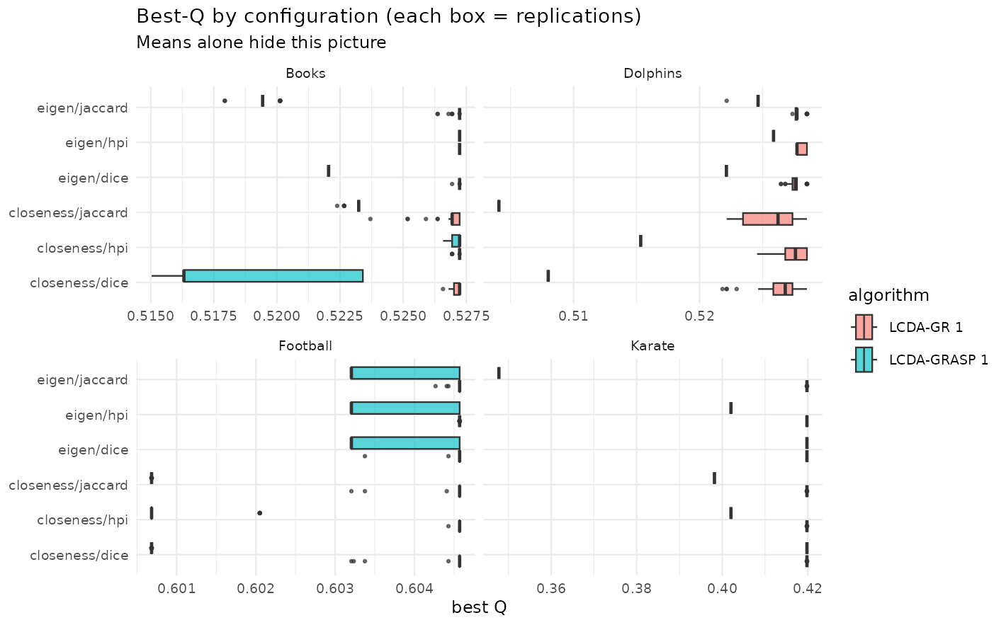

ggplot(res, aes(Q, colour = config)) +
  stat_ecdf(geom = "step", linewidth = 0.7) +
  facet_wrap(~ graph, scales = "free_x") +
  labs(title = "ECDF of best-Q by configuration", x = "Q", y = "F(Q)") +
  theme_minimal(base_size = 9) + theme(legend.position = "bottom")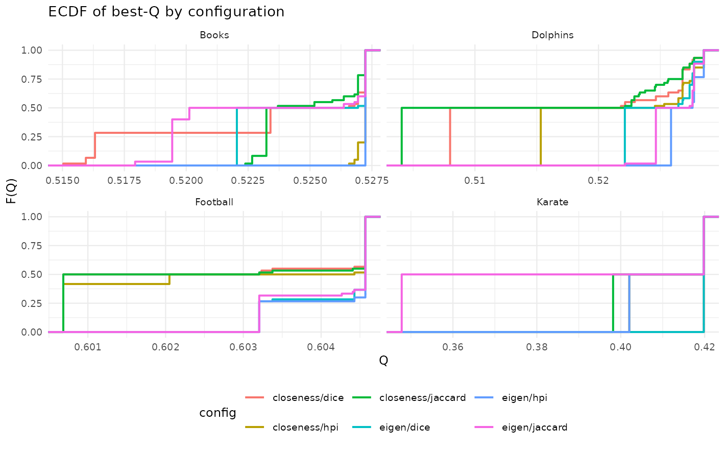

# Common Q scale (free_y), so the near-fixed Q reads as narrow vertical clouds
# instead of being auto-zoomed apart per panel.
ggplot(res, aes(Q, H, colour = algorithm, shape = similarity)) +
  geom_point(alpha = 0.6, size = 1.4) +
  facet_wrap(~ graph, scales = "free_y") +
  labs(title = "Joint (Q, H) across replicates",
       subtitle = "H varies within a narrow Q band: the near-tie regime where a lexicographic Q-then-H order could act") +
  theme_minimal(base_size = 9)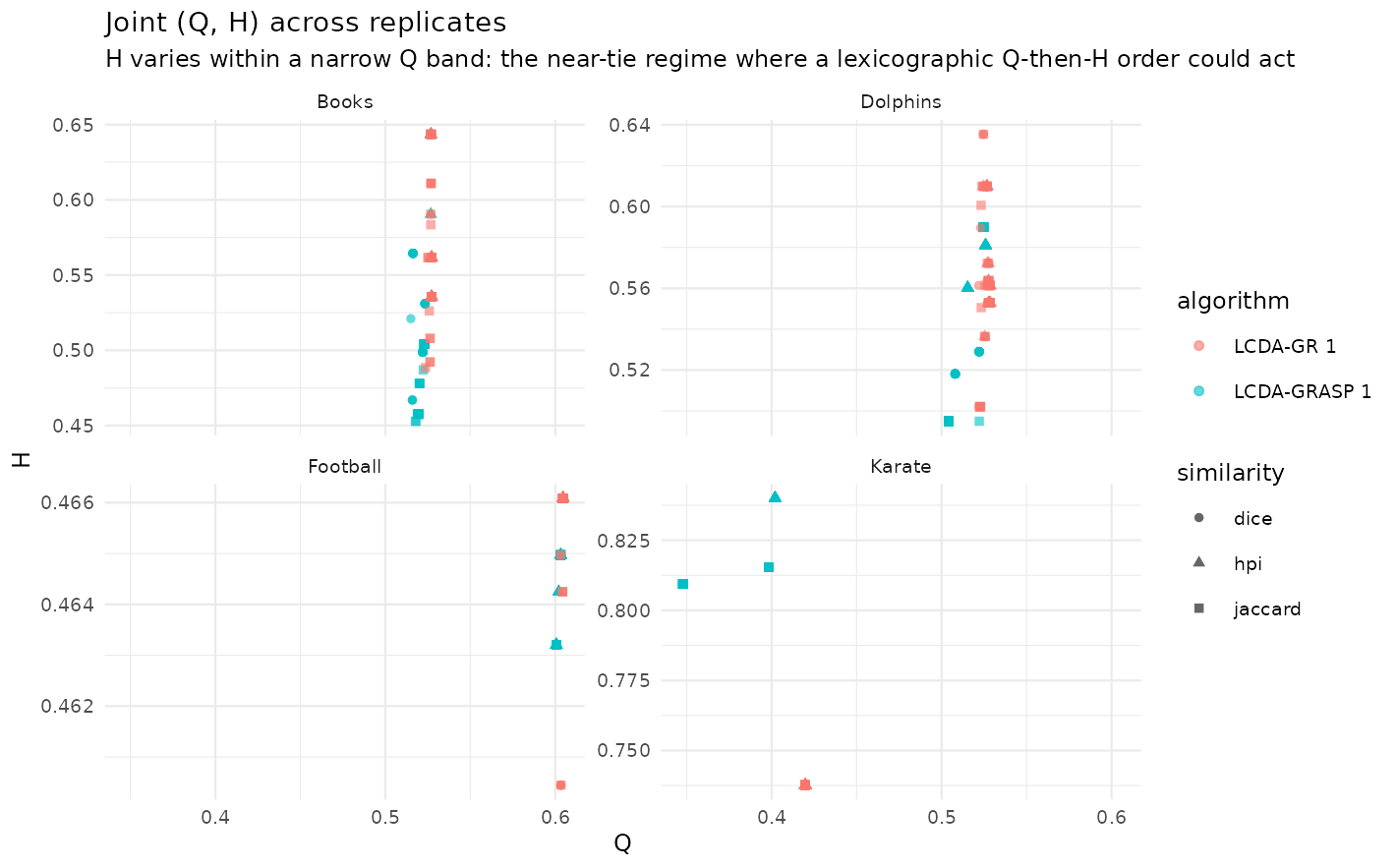

d_eda$results |>
  dplyr::group_by(graph, centrality, similarity) |>
  dplyr::summarise(Q = mean(Q), .groups = "drop_last") |>
  dplyr::slice_max(Q, n = 1) |>
  dplyr::ungroup() |>
  knitr::kable(digits = 4, caption = "Best centrality/similarity per network (mean Q).")

Best centrality/similarity per network (mean Q).
graph	centrality	similarity	Q
Books	closeness	hpi	0.5272
Books	eigen	hpi	0.5272
Dolphins	closeness	hpi	0.5214
Dolphins	eigen	hpi	0.5270
Football	closeness	hpi	0.6027
Football	eigen	hpi	0.6042
Karate	closeness	dice	0.4198
Karate	eigen	dice	0.4198

HPI + eigenvector is the modal winner, matching the paper’s recommendation — but the boxplots show the margins are often within noise, and the (Q, H) clouds are nearly vertical, i.e. $H$ varies at essentially fixed $Q$ . That is exactly the near-tie situation in which a lexicographic (Q, then H) objective could in principle bite. In practice it rarely does: $H$ seldom breaks a $Q$ -tie, as quantified in the Pool sensitivity article. The picture reinforces the same discipline as the LFR sweep — report the distribution, because the gap between configurations is frequently smaller than the within-configuration spread.

3. Modularity degeneracy and partition multiplicity

Modularity is an approximation, and one of its known pathologies is degeneracy: many structurally distinct partitions can have $Q$ within $\varepsilon$ of the maximum (Good, de Montjoye & Clauset 2010). For a multi-start metaheuristic this is double-edged — lots of optima to find, but the single partition you report (and therefore the leaders you name) is somewhat arbitrary. We audit how many distinct near-best partitions LCDA-GRASP finds and their mean pairwise NMI (low NMI = high degeneracy).

knitr::kable(
  dplyr::transmute(d_deg$results, graph, epsilon,
                   Q_star = round(Q_star, 4),
                   runs_in_band = n_runs_in_band,
                   distinct_partitions = n_distinct_partitions,
                   mean_NMI = round(mean_pairwise_NMI, 3)),
  caption = "Distinct near-best partitions and their similarity, per network and tolerance.")

Distinct near-best partitions and their similarity, per network and tolerance.
graph	epsilon	Q_star	runs_in_band	distinct_partitions	mean_NMI
karate	0.001	0.4020	33	1	1.000
karate	0.005	0.4020	33	1	1.000
karate	0.010	0.4020	33	1	1.000
karate	0.020	0.4020	33	1	1.000
dolphins	0.001	0.5259	4	1	1.000
dolphins	0.005	0.5259	12	3	0.845
dolphins	0.010	0.5259	28	6	0.821
dolphins	0.020	0.5259	59	13	0.798
polbooks	0.001	0.5272	44	2	0.980
polbooks	0.005	0.5272	48	4	0.967
polbooks	0.010	0.5272	60	6	0.931
polbooks	0.020	0.5272	60	6	0.931
sbm_polblogs_like	0.001	0.2286	1	1	NA
sbm_polblogs_like	0.005	0.2286	1	1	NA
sbm_polblogs_like	0.010	0.2286	8	8	0.458
sbm_polblogs_like	0.020	0.2286	29	29	0.427

ggplot(d_deg$results, aes(factor(epsilon), n_distinct_partitions, fill = graph)) +
  geom_col(position = "dodge") +
  labs(title = "Distinct near-best partitions within Q* − epsilon",
       x = expression(epsilon), y = "number of distinct partitions") +
  theme_minimal(base_size = 10)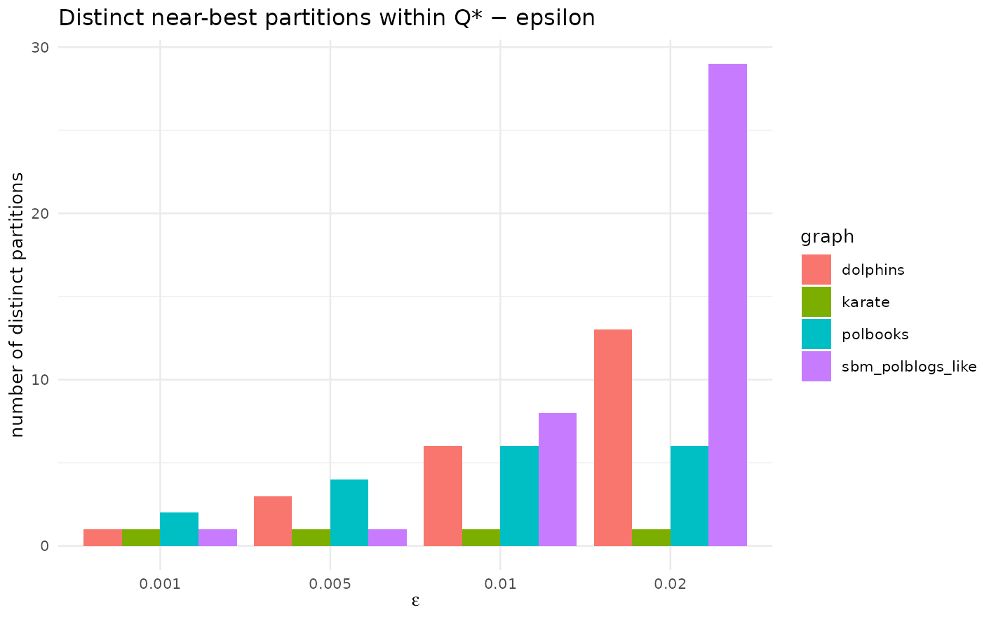

Even at small $\varepsilon$ , several distinct partitions coexist in the top band on the larger/diffuse networks, and the mean pairwise NMI sits below 1 — so the reported leader-community configuration is one of several near-equivalent ones. This does not invalidate the method, but it bounds the interpretability claim about “named leaders”: the names can shift across seeds. Beyond the well-known resolution limit, this near-optimum degeneracy is a genuine caveat for any modularity-maximising leader assignment and is worth reporting alongside it.

Taking the three together

The same lesson recurs at every scale of the analysis. As communities weaken, recovery falls and LCDA trails the strongest baselines while remaining competitive and matching ECG-style ensembles; across replicates the configuration margins are often inside the noise; and at the top of the $Q$ -landscape several partitions are statistically interchangeable, so the “named leaders” are not unique. None of this sinks the method — but it is the honest envelope around the headline numbers, and it is the reason the package reports distributions, leader-utility comparisons, and degeneracy counts rather than point estimates alone.

Reproducibility and data provenance

Every figure here is read from datasets shipped with the package; nothing is simulated at build time. Each dataset records the package version that generated it (not necessarily the version you installed: the generators are re-run only when the algorithms change), the release it first shipped in, and a SHA-256 checksum matching inst/extdata/SHA256SUMS:

do.call(rbind, lapply(c("lfr_robustness", "eda_replicates", "degeneracy"),
                      lcda_provenance))
#>          dataset generated_by generated_on first_release shipped_in
#> 1 lfr_robustness        0.3.1   2026-06-01         0.3.1      0.3.2
#> 2 eda_replicates        0.3.1   2026-05-31         0.3.1      0.3.2
#> 3     degeneracy        0.3.1   2026-05-31         0.3.1      0.3.2
#>                                                             sha256
#> 1 255da4a8af35fcb90173eb1e52ed931dbf4deba9c436b873724d5619506c599e
#> 2 4ae5d53c96d4962cc18ec7d4605a6a61197acdb15ce92b4ee29d8816f5ded28e
#> 3 2d94a87c44287c36f726b61ab377bac19ae97a3faa3612bab2da6dc785777b1b

Regenerate with data-raw/30_lfr_robustness.R, data-raw/70_eda.R and data-raw/60_degeneracy.R (each fixes a single documented seed; the LFR sweep uses $n = 500$ with 10 graphs per mixing level).

Scope. All synthetic results are at $n = 500$ (size effects are studied separately in the large-scale evaluation); recovery is reported as a mean with dispersion over the replicate graphs, never as a single number.

References

Good, B. H., de Montjoye, Y.-A., & Clauset, A. (2010). Performance of modularity maximization in practical contexts. Phys. Rev. E, 81, 046106. doi:10.1103/PhysRevE.81.046106
Lancichinetti, A., Fortunato, S., & Radicchi, F. (2008). Benchmark graphs for testing community detection algorithms. Phys. Rev. E, 78, 046110. doi:10.1103/PhysRevE.78.046110
Newman, M. E. J., & Girvan, M. (2004). Finding and evaluating community structure in networks. Phys. Rev. E, 69, 026113. doi:10.1103/PhysRevE.69.026113
Poulin, V., & Théberge, F. (2019). Ensemble clustering for graphs. Applied Network Science, 4, 51. doi:10.1007/s41109-019-0162-z ```