Plot a fitted LCDA result as a community-and-leader map

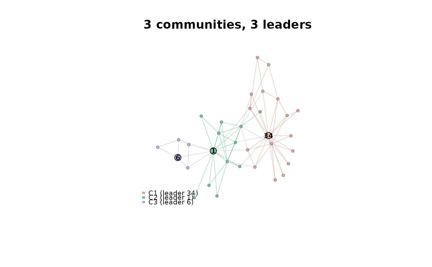
`plot()` methods for the objects returned by [lcda_grasp()], [lcda_gr()] and [lcda_ecg()]. The result carries the graph it was fitted on, so `plot(res)` is enough; pass a graph as the second argument to draw the same partition on a different graph over the same vertex set.

Usage

# S3 method for class 'lcda_grasp_result'
plot(x, y = NULL, ...)

# S3 method for class 'lcda_gr_result'
plot(x, y = NULL, ...)

# S3 method for class 'lcda_ecg_result'
plot(x, y = NULL, ...)

Arguments

x

a fitted `lcda_grasp_result`, `lcda_gr_result` or `lcda_ecg_result`.

y

optional [igraph::igraph] to draw on, with the same vertex set; defaults to the graph stored in `x`. It is simplified before drawing, as described above.

...

further arguments passed to [plot_partition()].

Value

invisibly, a list with the `layout` used and the community `colors`.

What is drawn

The stored `x$graph` is the graph **as the kernels saw it**: [as_csr()] collapses multi-edges, so a multigraph is drawn (and was optimised) as its simple counterpart. Passing your own graph as `y` does not change that; it too is simplified before drawing, so that the figure always shows the graph the modularity was computed on. Vertex count and vertex order are preserved, only parallel edges are merged.

See also

[plot_partition()], [lcda_plot_communities()], [lcda_metrics()].

Examples

g <- igraph::make_graph("Zachary")
res <- lcda_grasp(g, B = 20, seed = 1)
set.seed(1)
plot(res)