Tabular CUSUM control chart

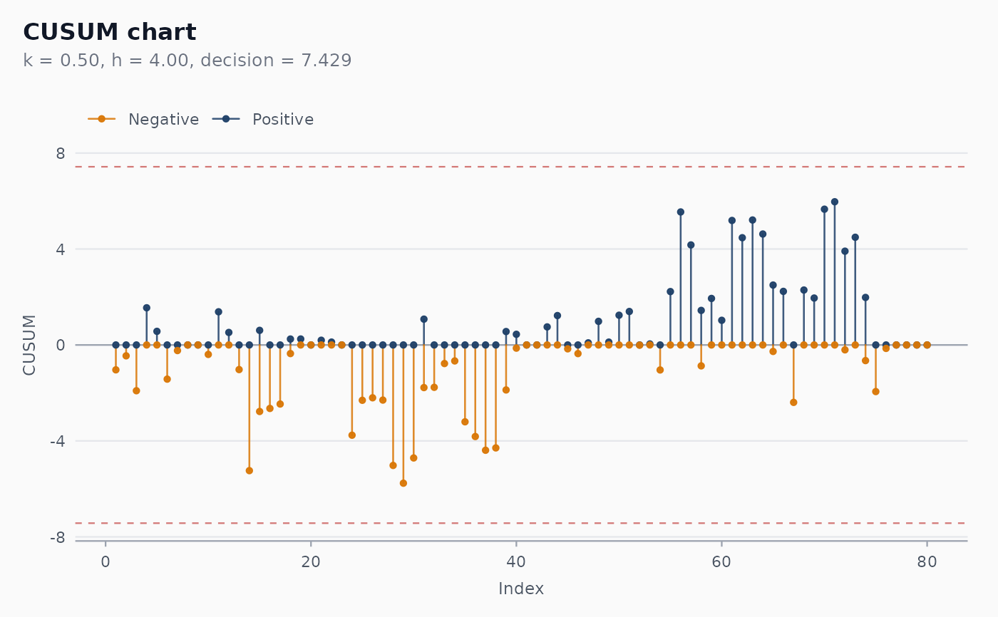
Constructs a two-sided tabular CUSUM chart for a single column of individual measurements. Two cumulative statistics, C+ (upward) and C- (downward), are accumulated against a target with a reference value k; an alarm fires when either crosses the decision interval h * sigma.

Usage

shewhart_cusum(
  data,
  value,
  index = NULL,
  target = NULL,
  sigma = NULL,
  k = 0.5,
  h = 4,
  locale = getOption("shewhart.locale", "en"),
  verbose = NULL
)

Arguments

data

A data frame.

value

Tidy-eval column reference for the measurement.

index

Optional tidy-eval column reference for the x-axis.

target

Numeric. Process target. Defaults to mean(value).

sigma

Numeric. Process sigma. Defaults to MR_bar / 1.128.

k

Numeric. Reference value in units of sigma. Default 0.5, tuned to detect 1-sigma shifts.

h

Numeric. Decision interval in units of sigma. Default 4, giving ARL_0 ~ 168 for k = 0.5. Use h = 5 for ARL_0 ~ 465 (Hawkins & Olwell 1998).

locale

One of "en", "pt", "es", "fr".

verbose

Logical. Print progress messages?

Value

A shewhart_chart object of subclass shewhart_cusum. The augmented slot has columns .value, .cusum_pos, .cusum_neg (the two accumulated statistics, both non-negative), .upper (the decision interval h * sigma), and .flag_signal.

Details

By default, sigma is estimated from the moving range of value (MR_bar / 1.128); the target is the mean of value. Either can be overridden via target and sigma for Phase II monitoring against pre-calibrated values.

References

Page, E. S. (1954). Continuous Inspection Schemes. Biometrika, 41(1-2), 100-115. doi:10.1093/biomet/41.1-2.100

Hawkins, D. M., & Olwell, D. H. (1998). Cumulative Sum Charts and Charting for Quality Improvement. Springer.

Montgomery, D. C. (2019). Introduction to Statistical Quality Control (8th ed.). Wiley. Chapter 9.

Examples

set.seed(1)
df <- data.frame(
  day = 1:80,
  y   = c(rnorm(40, mean = 100, sd = 2),
          rnorm(40, mean = 101, sd = 2))   # 0.5 sigma shift
)
fit <- shewhart_cusum(df, value = y, index = day)
print(fit)
#> 
#> ── Shewhart chart cusum ────────────────────────────────────────────────────────
#> • Observations / subgroups: 80
#> • Phase: "phase_1"
#> • Sigma estimate ("mr"): 1.857
#> 
#> ── Control limits ──
#> 
#> # A tibble: 2 × 3
#>   chart line    value
#>   <chr> <chr>   <dbl>
#> 1 CUSUM h_upper  7.43
#> 2 CUSUM h_lower -7.43
#> ── Rule violations ──
#> 
#> ✔ No violations across 1 rule: "cusum_decision".
# \donttest{
ggplot2::autoplot(fit)

# }