Memory-based charts: EWMA and CUSUM
Source:vignettes/memory-based-charts.Rmd
memory-based-charts.RmdWhen the Shewhart chart is too slow
A Shewhart chart looks at one observation at a time. Each point is compared against the centre line and the 3-sigma limits, and that’s it — the chart has no memory of what came before (the runs rules add a little, but only a little). This makes Shewhart charts excellent at catching large shifts the moment they happen, but fairly slow at catching small persistent shifts that would only become visible after the data has had time to drift.
EWMA and CUSUM accumulate information across observations, trading a slightly less direct interpretation for substantially better sensitivity to small shifts.
# A 0.5-sigma sustained shift after observation 40
set.seed(2026)
n      <- 80
shift  <- c(rnorm(40, mean = 0, sd = 1),
            rnorm(40, mean = 0.5, sd = 1))
df     <- tibble::tibble(t = seq_len(n), y = shift)

imr  <- shewhart_i_mr(df,  value = y, index = t)
ewma <- shewhart_ewma(df,  value = y, index = t)
cusum <- shewhart_cusum(df, value = y, index = t)

# Position of the first alarm under each chart
first_alarm <- function(fit) {
  hits <- which(fit$augmented$.flag_any)
  if (length(hits) == 0L) NA_integer_ else min(hits)
}
tibble::tibble(
  chart  = c("I-MR", "EWMA", "CUSUM"),
  alarm  = c(first_alarm(imr), first_alarm(ewma), first_alarm(cusum))
)
#> # A tibble: 3 × 2
#>   chart alarm
#>   <chr> <int>
#> 1 I-MR     10
#> 2 EWMA     NA
#> 3 CUSUM    15
For a 0.5-sigma shift, the I-MR chart often fails to signal at all within 80 observations, while the EWMA and CUSUM typically catch it within a few points of the change.
EWMA — Exponentially Weighted Moving Average
The EWMA statistic is a recursive convex combination:
With lambda close to 1 the chart behaves like a Shewhart
I chart (little memory). With lambda close to 0 it averages
over a long history (heavy memory, slow but very sensitive). The
classical default lambda = 0.2, L = 2.7 gives
ARL_0 ≈ 370 and is well matched to detecting shifts of 0.5
to 1 sigma (Lucas & Saccucci 1990).
fit <- shewhart_ewma(df, value = y, index = t,
                     lambda = 0.2, L = 2.7)
fit
#>
#> ── Shewhart chart ewma ─────────────────────────────────────────────────────────
#> • Observations / subgroups: 80
#> • Phase: "phase_1"
#> • Sigma estimate ("mr"): 1.014
#>
#>
#> ── Control limits ──
#> # A tibble: 3 × 3
#>   chart line            value
#>   <chr> <chr>           <dbl>
#> 1 EWMA  CL              0.165
#> 2 EWMA  UCL_asymptotic  1.08
#> 3 EWMA  LCL_asymptotic -0.748
#> ── Rule violations ──
#>
#> ✔ No violations across 1 rule: "nelson_1_beyond_3s".
autoplot(fit)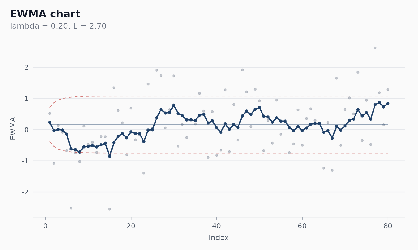
The control limits in an EWMA chart are time-varying
by default. They start narrow and widen out to the asymptotic value
L · σ · sqrt(λ / (2 - λ)) as the recursion warms up. This
is the correct probability-symmetric calibration; setting
steady_state = TRUE flattens them out at the asymptotic
value (a common simplification once you have a long enough
baseline).
shewhart_ewma(df, value = y, index = t, steady_state = TRUE) |>
  autoplot()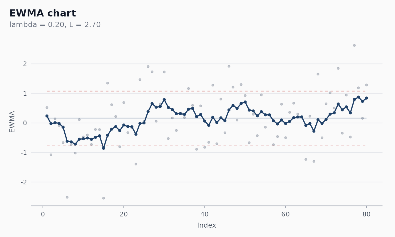
Choosing lambda
A practical guide (Montgomery 2019, Table 9.10):
| Target shift size | Reasonable lambda
|
L |
ARL_0 |
|---|---|---|---|
| 0.25 σ | 0.05 | 2.49 | ~370 |
| 0.50 σ | 0.10 | 2.70 | ~370 |
| 0.75 σ | 0.20 | 2.86 | ~370 |
| 1.00 σ | 0.40 | 3.00 | ~370 |
Choose the smallest shift you care about, then use the
matching row. You can validate the actual ARL with
[shewhart_arl()] from the arl-simulation vignette.
CUSUM — Cumulative Sum
The tabular CUSUM keeps two non-negative running totals, one for upward drift and one for downward drift:
An alarm fires when either crosses the decision
interval h · sigma. The reference value
k is typically half the smallest shift size the
chart should be sensitive to (so k = 0.5 for shifts of
1·σ); h controls the false-alarm rate.
fit <- shewhart_cusum(df, value = y, index = t, k = 0.5, h = 4)
fit
#>
#> ── Shewhart chart cusum ────────────────────────────────────────────────────────
#> • Observations / subgroups: 80
#> • Phase: "phase_1"
#> • Sigma estimate ("mr"): 1.014
#>
#>
#> ── Control limits ──
#> # A tibble: 2 × 3
#>   chart line    value
#>   <chr> <chr>   <dbl>
#> 1 CUSUM h_upper  4.05
#> 2 CUSUM h_lower -4.05
#> ── Rule violations ──
#>
#> ! 1 violation across 1 rule.
#> cusum_decision: 1 hit.
autoplot(fit)
The plot draws C+ as positive bars (potential upward
drift) and C- as negative bars (potential downward drift),
with the symmetric decision interval in dashed red. CUSUM’s main charm
is interpretability once it signals: the bar’s height tells you how much
accumulated deviation triggered the alarm.
Choosing k and h
Hawkins & Olwell (1998), Table 3.1, gives ARL profiles for
k = 0.5 (the most common choice):
h |
ARL_0 (in control) | ARL_1 at 1σ shift |
|---|---|---|
| 4.00 | ~168 | ~8.4 |
| 4.77 | ~370 | ~10.4 |
| 5.00 | ~465 | ~10.9 |
The default h = 4 is appropriate for diagnostic
monitoring. For a production chart matched to the typical Shewhart
ARL_0 = 370, raise h to 4.77.
Phase II monitoring
Both charts accept target and sigma to
override the in-data estimates — exactly what you need for Phase II
monitoring against a clean Phase I baseline. The example below
calibrates on a 60-point in-control baseline and then monitors a fresh
40-point period:
set.seed(1)
baseline <- tibble::tibble(t = 1:60, y = rnorm(60, mean = 100, sd = 2))
mu_hat   <- mean(baseline$y)
sd_hat   <- sd(baseline$y)

new_data <- tibble::tibble(
  t = 61:100,
  y = rnorm(40, mean = 100.8, sd = 2)   # 0.4 sigma shift
)

shewhart_ewma(new_data, value = y, index = t,
              target = mu_hat, sigma = sd_hat,
              lambda = 0.2, L = 2.7) |>
  autoplot()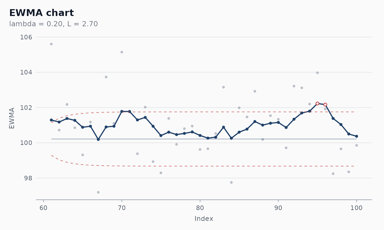
A calibrate() / monitor() integration for
memory-based charts is on the roadmap for a future release; for the
moment the explicit target / sigma arguments
give you the same workflow with one extra line.
Which one should I use?
| Question | EWMA | CUSUM | Shewhart |
|---|---|---|---|
| Best at 0.25–1 σ shifts? | ✔ | ✔ | |
| Best at >2 σ shifts? | ✔ | ||
| Plot reads like the original variable? | ✔ | ✔ | |
| Communicates magnitude of accumulated drift? | ✔ | ||
| Survives autocorrelated data well? | (with care) | (with care) | |
| Pairs naturally with runs rules? | (Nelson 1 only) | ✔ |
Many practitioners run both a Shewhart chart and an EWMA (or CUSUM) on the same series — the Shewhart catches large excursions, the memory-based catches the slow drifts.
References
- Roberts, S. W. (1959). Control Chart Tests Based on Geometric Moving Averages. Technometrics, 1(3), 239-250.
- Page, E. S. (1954). Continuous Inspection Schemes. Biometrika, 41(1-2), 100-115.
- Lucas, J. M., & Saccucci, M. S. (1990). Exponentially Weighted Moving Average Control Schemes: Properties and Enhancements. Technometrics, 32(1), 1-12.
- Hawkins, D. M., & Olwell, D. H. (1998). Cumulative Sum Charts and Charting for Quality Improvement. Springer.
- Montgomery, D. C. (2019). Introduction to Statistical Quality Control (8th ed.). Wiley. Chapter 9.