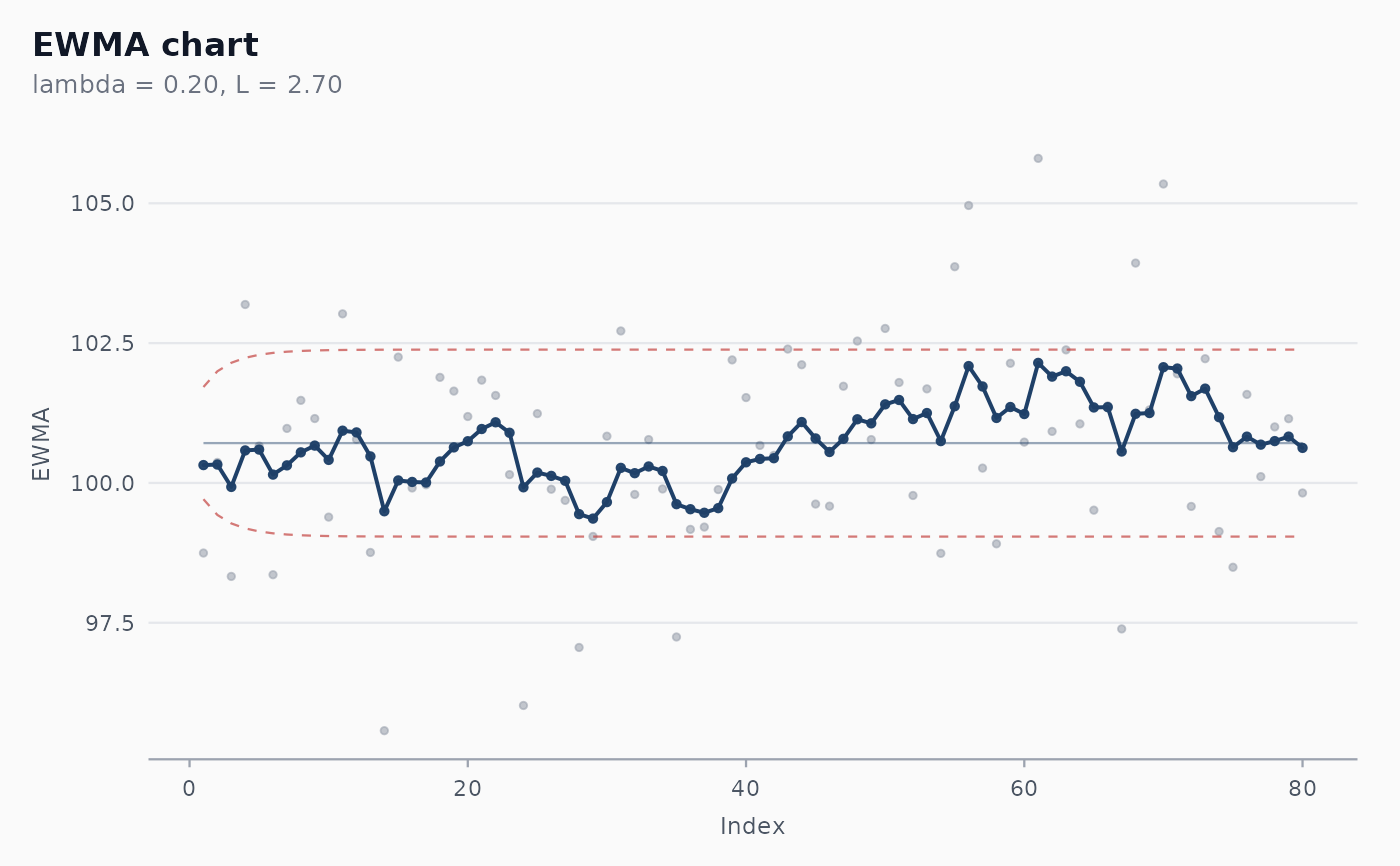
Exponentially Weighted Moving Average (EWMA) control chart

Constructs an EWMA chart for a single column of individual measurements. The chart is more sensitive than a Shewhart I chart to small but persistent shifts in the process mean, at the cost of a longer reaction time to large shifts.

Usage

shewhart_ewma(
  data,
  value,
  index = NULL,
  target = NULL,
  sigma = NULL,
  lambda = 0.2,
  L = 2.7,
  steady_state = FALSE,
  rules = "nelson_1_beyond_3s",
  locale = getOption("shewhart.locale", "en"),
  verbose = NULL
)

Arguments

data: A data frame.
value: Tidy-eval column reference for the measurement.
index: Optional tidy-eval column reference for the x-axis.
target: Numeric. Process target / centre line. Defaults to mean(value).
sigma: Numeric. Process sigma. Defaults to MR_bar / 1.128.
lambda: Numeric in (0, 1]. Smoothing constant. Default 0.2. Smaller lambda = more memory, more sensitive to small shifts.
L: Numeric. Width of the limits in standard errors of the EWMA. Default 2.7, which combined with lambda = 0.2 yields ARL_0 ~ 370 (Lucas & Saccucci 1990).
steady_state: Logical. Use asymptotic (constant) limits instead of time-varying ones?
rules: Character vector of runs rules to flag. Defaults to Nelson 1 only — the EWMA's own limits already encode most of the diagnostic power and the higher-order Nelson rules are not designed for autocorrelated statistics.
locale: One of "en", "pt", "es", "fr".
verbose: Logical. Print progress messages?

Value

A shewhart_chart object of subclass shewhart_ewma. The augmented slot has columns .value (the original observation), .ewma (the smoothed statistic z_i, plotted on the chart), and the usual .center, .upper, .lower, .flag_*.

Details

By default, sigma is estimated from the moving range of value (Wheeler 1992 convention, MR_bar / 1.128); the centre is the mean of value. Either can be overridden via target and sigma for Phase II monitoring against pre-calibrated values.

Limits are time-varying by default — they widen out from target as the EWMA "warms up" — converging to the asymptotic limits as i -> infinity. Set steady_state = TRUE to use the asymptotic limits everywhere (commonly chosen when calibrating from a long baseline).

References

Roberts, S. W. (1959). Control Chart Tests Based on Geometric Moving Averages. Technometrics, 1(3), 239-250. doi:10.1080/00401706.1959.10489860

Lucas, J. M., & Saccucci, M. S. (1990). Exponentially Weighted Moving Average Control Schemes: Properties and Enhancements. Technometrics, 32(1), 1-12. doi:10.1080/00401706.1990.10484583

Montgomery, D. C. (2019). Introduction to Statistical Quality Control (8th ed.). Wiley. Chapter 9.

Examples

set.seed(1)
df <- data.frame(
  day = 1:80,
  y   = c(rnorm(40, mean = 100, sd = 2),
          rnorm(40, mean = 101, sd = 2))   # 0.5 sigma shift
)
fit <- shewhart_ewma(df, value = y, index = day)
print(fit)
#> 
#> ── Shewhart chart ewma ─────────────────────────────────────────────────────────
#> • Observations / subgroups: 80
#> • Phase: "phase_1"
#> • Sigma estimate ("mr"): 1.857
#> 
#> ── Control limits ──
#> 
#> # A tibble: 3 × 3
#>   chart line           value
#>   <chr> <chr>          <dbl>
#> 1 EWMA  CL             101. 
#> 2 EWMA  UCL_asymptotic 102. 
#> 3 EWMA  LCL_asymptotic  99.0
#> ── Rule violations ──
#> 
#> ✔ No violations across 1 rule: "nelson_1_beyond_3s".
# \donttest{
ggplot2::autoplot(fit)

# }