Hotelling T-squared multivariate control chart

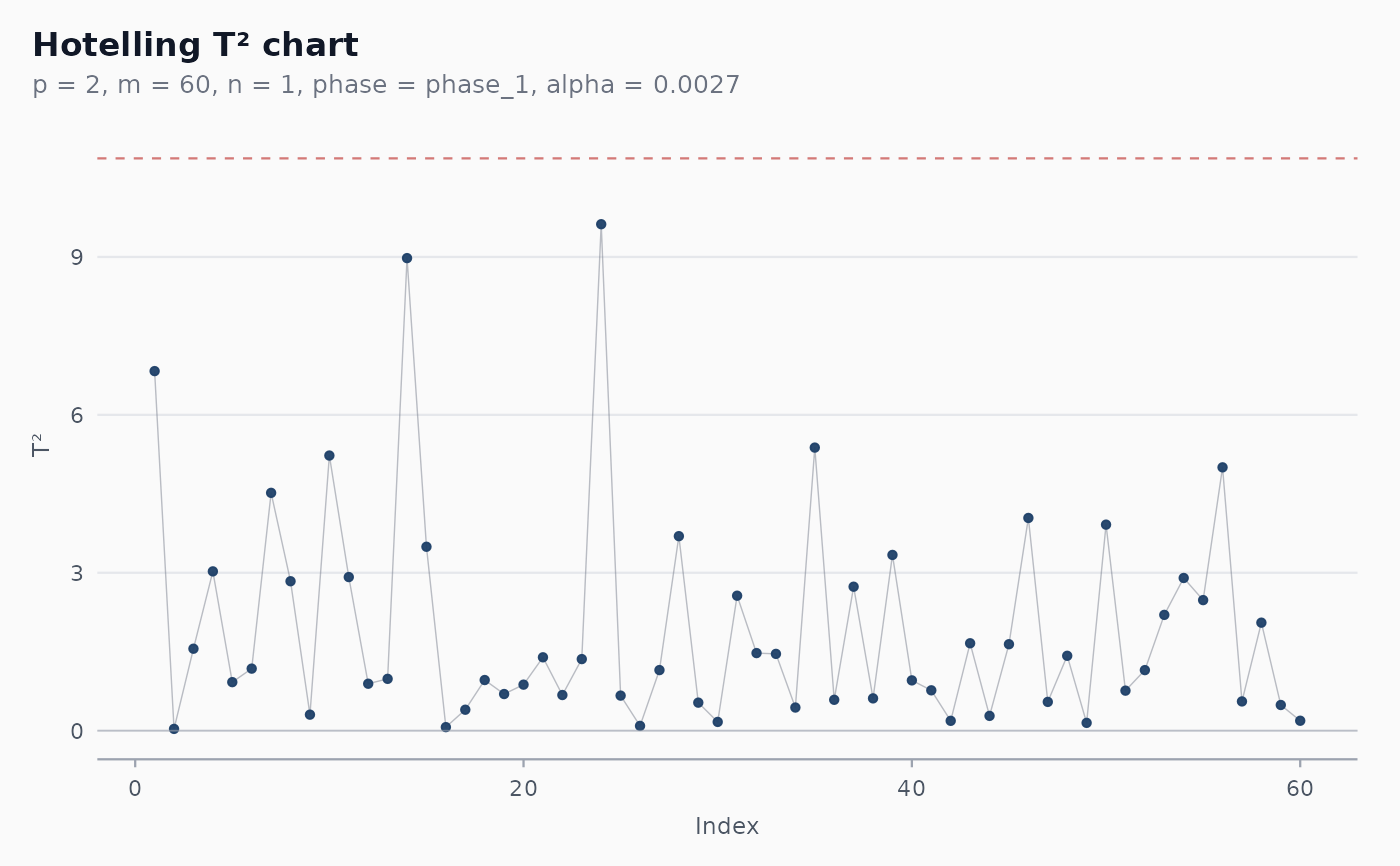
Constructs a Hotelling T² chart for joint monitoring of p correlated quality characteristics. Use this chart when the variables genuinely co-vary — a classical example is a chemical process where temperature, pressure and flow rate are mechanically coupled, and a fault that breaks the coupling moves them off the joint distribution but possibly stays inside each marginal limit.

Usage

shewhart_hotelling(
  data,
  vars,
  subgroup = NULL,
  index = NULL,
  phase = c("phase_1", "phase_2"),
  alpha = 0.0027,
  locale = getOption("shewhart.locale", "en"),
  verbose = NULL
)

Arguments

data

A data frame.

vars

Tidy-select expression for the columns containing the variables to monitor jointly (c(x1, x2, x3), tidyselect::starts_with("temp"), etc.). Must select at least 2 columns.

subgroup

Optional tidy-eval column for rational subgrouping. If supplied, all rows sharing a value of this column are treated as a single subgroup. If NULL (default), every row is its own observation (individual-observations chart).

index

Optional tidy-eval column for the x-axis. If supplied, must vary across observations (or across subgroups, if subgroup is supplied).

phase

One of "phase_1" (default; retrospective) or "phase_2" (prospective monitoring of new observations against parameters estimated from the same data).

alpha

Type-I error rate per observation. Default 0.0027, matching the conventional Shewhart 3-sigma false-alarm rate.

locale

One of "en", "pt", "es", "fr".

verbose

Logical. Print progress messages?

Value

A shewhart_chart object of subclass shewhart_hotelling. The augmented tibble has columns .t2 (the statistic), .upper (UCL — constant within a chart), .flag_signal and .flag_any, and one .contrib_<var> column per monitored variable giving that variable's marginal contribution to the alarm (Mason et al. 1995). The limits slot contains the chart-level UCL; the metadata slot stores the variable names, subgroup column name, and the parameters p, m, n, phase, alpha that determined the limit.

Details

Both individual observations (subgroup = NULL) and rationally subgrouped observations (subgroup supplied) are supported. The chart selects the appropriate exact small-sample limits for the selected phase (Phase I uses retrospective limits derived from a Beta or F distribution; Phase II uses the slightly wider limits that propagate the Phase I parameter uncertainty to a fresh observation).

References

Hotelling, H. (1947). Multivariate quality control. In: Techniques of Statistical Analysis. McGraw-Hill.

Tracy, N. D., Young, J. C., & Mason, R. L. (1992). Multivariate control charts for individual observations. Journal of Quality Technology, 24(2), 88-95. doi:10.1080/00224065.1992.11979383

Mason, R. L., Tracy, N. D., & Young, J. C. (1995). Decomposition of T² for multivariate control chart interpretation. Journal of Quality Technology, 27(2), 99-108. doi:10.1080/00224065.1995.11979573

Mason, R. L., & Young, J. C. (2002). Multivariate Statistical Process Control with Industrial Applications. SIAM/ASA.

Montgomery, D. C. (2019). Introduction to Statistical Quality Control (8th ed.). Wiley. Chapter 11.

Examples

set.seed(1)
Sigma <- matrix(c(1, 0.7, 0.7, 1), 2, 2)
Z     <- MASS::mvrnorm(60, c(0, 0), Sigma)
df    <- tibble::tibble(t = 1:60, x1 = Z[, 1], x2 = Z[, 2])
fit   <- shewhart_hotelling(df, vars = c(x1, x2), index = t)
print(fit)
#> 
#> ── Shewhart chart hotelling ────────────────────────────────────────────────────
#> • Observations / subgroups: 60
#> • Phase: "phase_1"
#> • Sigma estimate ("hotelling"): NA
#> 
#> ── Control limits ──
#> 
#> # A tibble: 1 × 3
#>   chart line  value
#>   <chr> <chr> <dbl>
#> 1 T2    UCL    10.9
#> ── Rule violations ──
#> 
#> ✔ No violations across 1 rule: "hotelling_ucl".
# \donttest{
ggplot2::autoplot(fit)

# }