Multivariate EWMA control chart

Constructs a multivariate Exponentially Weighted Moving Average (MEWMA) chart for jointly monitoring p correlated variables. The chart is more sensitive than the Hotelling T^2 chart to small persistent shifts in the vector mean, in the same way the univariate EWMA is more sensitive than a Shewhart I chart.

Usage

shewhart_mewma(
  data,
  vars,
  index = NULL,
  target = NULL,
  cov = NULL,
  lambda = 0.1,
  h = NULL,
  steady_state = FALSE,
  locale = getOption("shewhart.locale", "en"),
  verbose = NULL
)

Arguments

data

A data frame.

vars

Tidy-select expression for the columns to monitor jointly. Must select at least 2 columns.

index

Optional tidy-eval column for the x-axis.

target

Optional length-p numeric vector. The in-control mean. Defaults to colMeans(data[, vars]).

cov

Optional p x p covariance matrix. Defaults to cov(data[, vars]).

lambda

Smoothing constant in (0, 1]. Default 0.1.

h

Decision interval (UCL on the T^2 statistic). If NULL, looked up in the ARL_0 ~ 200 table matching steady_state.

steady_state

Logical. Use the steady-state covariance (lambda / (2 - lambda)) * Sigma everywhere instead of the time-varying form? Default FALSE.

locale

One of "en", "pt", "es", "fr".

verbose

Logical. Print progress messages?

Value

A shewhart_chart object of subclass shewhart_mewma. The augmented tibble has columns .t2 (the MEWMA statistic), .upper (the decision interval h), and .flag_signal.

Details

By default target (the in-control mean vector) and cov (the in-control covariance) are estimated from the data. For Phase II monitoring, supply both explicitly so the limits use the calibration values. The decision interval h is calibrated by lookup in a table giving ARL_0 ~ 200 (with known in-control parameters) for lambda in {0.05, 0.10, 0.20, 0.40} and p = 2..6. There is one table for each covariance mode and the lookup follows steady_state; the steady-state table reproduces Prabhu & Runger (1997). If the (lambda, p) combination is outside the tabulated range, the user must pass h explicitly.

In Phase II (monitor()), the recursion continues from the last Phase I vector Z (and from the previous batch when monitor() is chained), with the covariance of the continued recursion.

References

Lowry, C. A., Woodall, W. H., Champ, C. W., & Rigdon, S. E. (1992). A Multivariate Exponentially Weighted Moving Average Control Chart. Technometrics, 34(1), 46-53. doi:10.1080/00401706.1992.10485232

Prabhu, S. S., & Runger, G. C. (1997). Designing a Multivariate EWMA Control Chart. Journal of Quality Technology, 29(1), 8-15. doi:10.1080/00224065.1997.11979721

Examples

set.seed(1)
Sigma <- matrix(c(1, 0.6, 0.6, 1), 2, 2)
base  <- MASS::mvrnorm(60, c(0, 0), Sigma)
shift <- MASS::mvrnorm(40, c(0.4, 0.4), Sigma)         # 0.4 sigma shift
df    <- data.frame(t = 1:100,
                    x1 = c(base[, 1], shift[, 1]),
                    x2 = c(base[, 2], shift[, 2]))
fit <- shewhart_mewma(df, vars = c(x1, x2), index = t,
                      target = c(0, 0), cov = Sigma,
                      lambda = 0.1)
print(fit)
#> 
#> ── Shewhart chart mewma ────────────────────────────────────────────────────────
#> • Observations / subgroups: 100
#> • Phase: "phase_1"
#> • Sigma estimate ("mewma"): NA
#> 
#> ── Control limits ──
#> 
#> # A tibble: 1 × 3
#>   chart line  value
#>   <chr> <chr> <dbl>
#> 1 MEWMA UCL    8.76
#> ── Rule violations ──
#> 
#> ✔ No violations across 1 rule: "mewma_h".
# \donttest{
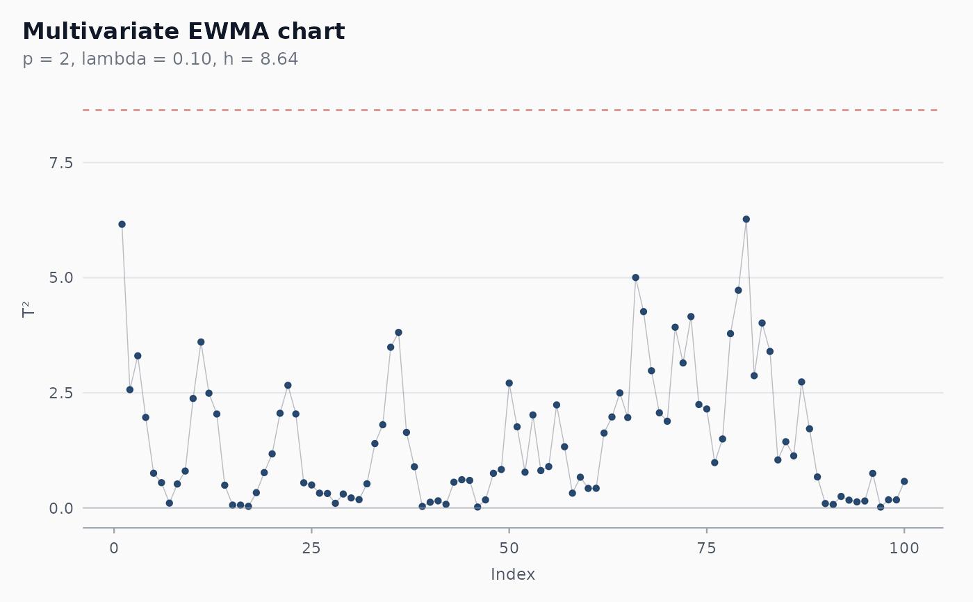
ggplot2::autoplot(fit)

# }