Regression-based control chart for processes with trend — shewhart

Fits a chosen model to the data (linear, log, log-log, Gompertz, logistic, or a user-supplied formula), then constructs control limits around the fitted curve using the moving-range estimator on the residuals (Wheeler 1992). Optionally detects phase changes automatically via runs tests on the residuals and re-fits each phase.

Usage

shewhart_regression(
  data,
  value,
  index,
  model = c("auto", "linear", "log", "loglog", "gompertz", "logistic"),
  formula = NULL,
  dummy = NULL,
  start_base = NULL,
  phase_changes = NULL,
  phase_rule = "nelson_2_nine_same",
  rules = c("nelson_1_beyond_3s", "nelson_2_nine_same"),
  sigma_method = c("mr", "median_mr", "biweight", "sd"),
  lower_bound = NA_real_,
  limits_scale = c("original", "model"),
  locale = getOption("shewhart.locale", "en"),
  verbose = NULL
)

Arguments

data: A data frame.
value: Tidy-eval column reference for the response.
index: Tidy-eval column reference for the predictor (typically time, but can be any continuous variable).
model: Character. One of "auto" (Box-Cox guidance), "linear", "log" (fits log(y + 1) ~ N), "loglog", "gompertz", "logistic". For full control, supply formula instead. With "auto", each phase gets the Box-Cox profile maximiser lambda of y + 1, rounded to the nearest rung of the ladder that the menu offers: lambda < 0.25 selects "log", any larger value selects "linear" (a square-root lambda near 0.5 has no dedicated model and maps to "linear"; "loglog" is a stronger transform than log and is never chosen automatically).
formula: Optional one-sided or two-sided formula referencing columns in data. If provided, overrides model. The model may reference .N, the position of the observation within its phase. When the left-hand side is a recognised transformation of the response – log(y), log(y + c), log(y, base), log10(), log2(), log1p() or sqrt(), optionally wrapped in I() – the fitted values are back-transformed to the scale of the data and limits_scale = "model" is available.
dummy: Optional tidy-eval column reference for an additive covariate (a "dummy" in the original v0.1 nomenclature; can be any factor or numeric covariate the user wants to adjust for, such as day-of-week effects or treatment indicators).
start_base: Integer or NULL. Number of initial observations used to estimate the first (base) phase. With automatic phase detection, NULL (the default) means 10. When phase_changes is supplied, NULL means the base phase ends just before the first supplied change; an explicit start_base adds a cut at observation start_base + 1 in addition to phase_changes.
phase_changes: Optional vector of index values at which to force a phase change (the observation whose index equals the value starts the new phase). If NULL, phase changes are detected automatically using the supplied phase_rule. A zero-length vector (e.g. integer(0)) fits a single phase without detection; it then needs only 3 observations, which is what a prospective replay needs to calibrate one phase at a time (see Details).
phase_rule: Character. Runs rule used to detect new phases. See shewhart_rules_available(). Default Nelson 2 (9 points same side; ARL_0 = 2^9 - 1 = 511). For backward compatibility with v0.1.x, use "we_seven_same" (7 points; ARL_0 = 2^7 - 1 = 127).
rules: Character vector of rules to flag on the final chart.
sigma_method: One of "mr" (default), "median_mr", "biweight" (Tukey-style robust), or "sd".
lower_bound: Numeric scalar or NA. If non-NA, lower limit is clipped at this value (commonly 0 for counts). Default NA (no clipping). Stored in metadata and honoured by monitor().
limits_scale: Scale on which the limits are built. With "original" (default), sigma is estimated from the residuals on the scale of the data and the band fitted +- 3 sigma is symmetric. With "model", sigma is estimated from the moving ranges of the residuals on the transformed scale of the model's left-hand side g(y); the band g_hat +- 3 sigma is formed there and centre line and limits are back-transformed with g^-1. With model = "log" this gives the multiplicative, asymmetric bands of Perla et al. (2020) and Ferraz et al. (2020) – an individuals chart on the residuals of log(1 + y) ~ t – whose lower limit never falls below 0. For models whose left-hand side is the raw response ("linear", "gompertz", "logistic", or a formula such as y ~ .N) the two options coincide. With "model", the .sigma column of the augmented tibble (and metadata$phase_sigma, sigma_hat) is on the model scale, and two extra columns hold what the runs rules are applied to: .model_value (the transformed observation g(y)) and .model_center (the fitted value g_hat).
locale: Character. One of "en", "pt", "es", "fr".
verbose: Logical. Print progress messages?

Value

A shewhart_chart object of subclass shewhart_regression. The fits slot contains a list of fitted model objects (one per phase; a phase with fewer than 3 observations reuses the previous phase's fit). The metadata slot additionally stores phase_n_end (the last within-phase position .N reached by each phase's fit) and phase_sigma (the residual sigma of each phase), which monitor() uses to extrapolate the last phase, together with limits_scale and lower_bound. The sigma_hat slot is the median of the per-phase sigmas.

The .phase_label column names the phases "Base", "Phase 1", ..., "Monitoring" (localised). When the index column is a Date (or a date-time), every phase but the last also carries its end date, e.g. "Base (until 2020-05-11)". The first index value of each phase is the date on which it starts.

Details

This is the package's flagship chart, intended for trended or non-stationary processes for which classical Shewhart charts give systematically wrong limits. See the vignette regression-charts for a thorough discussion and examples.

Models that take the logarithm of the response ("log", "loglog", and "auto" whenever it selects "log") require non-negative values: log(1 + y) is undefined for a negative count such as a bulletin that revises a cumulative total downwards. The function stops with an error naming the offending row instead of returning NaN limits; filter or reconcile such rows first.

A Phase I chart refits every phase, including the last one (labelled "Monitoring"). To judge new observations against the limits of the last phase projected forward, as in a prospective analysis, calibrate on the data up to the end of the last phase with calibrate() and pass the rest to monitor(): it continues .N, uses the stored sigma, and honours limits_scale and lower_bound. A prospective replay in the manner of Ferraz et al. (2020) chains these steps one phase at a time: calibrate a single phase (phase_changes = integer(0)) on its first observations, monitor the rows that follow, and start the next phase at the first index after the first run flagged by "we_seven_same" (column .flag_we_seven_same of the monitored chart, with rules = "we_seven_same").

References

Mandel, B. J. (1969). The Regression Control Chart. Journal of Quality Technology, 1(1), 1-9. doi:10.1080/00224065.1969.11980341

Wheeler, D. J., & Chambers, D. S. (1992). Understanding Statistical Process Control (2nd ed.). SPC Press.

Perla, R. J., Provost, S. M., Parry, G. J., Little, K., & Provost, L. P. (2020). Understanding variation in reported COVID-19 deaths with a novel Shewhart chart application. International Journal for Quality in Health Care, 32(10), 685-688. doi:10.1093/intqhc/mzaa069

Ferraz, C., Petenate, A. J., Leite Wanderley, A., Ospina, R., Torres, J., & Peruzzi Moreira, A. (2020). COVID-19: monitoramento por graficos de Shewhart. Revista Brasileira de Estatistica, 78(245), 23-41.

Box, G. E. P., & Cox, D. R. (1964). An Analysis of Transformations. Journal of the Royal Statistical Society, Series B, 26(2), 211-252. doi:10.1111/j.2517-6161.1964.tb00553.x

Examples

# \donttest{
set.seed(1)
df <- data.frame(
  t = 1:60,
  y = c(1:30 * 0.5 + rnorm(30, sd = 0.5),    # phase 1: linear trend
        15 + 1:30 * 0.1 + rnorm(30, sd = 0.5)) # phase 2: shift + slowdown
)
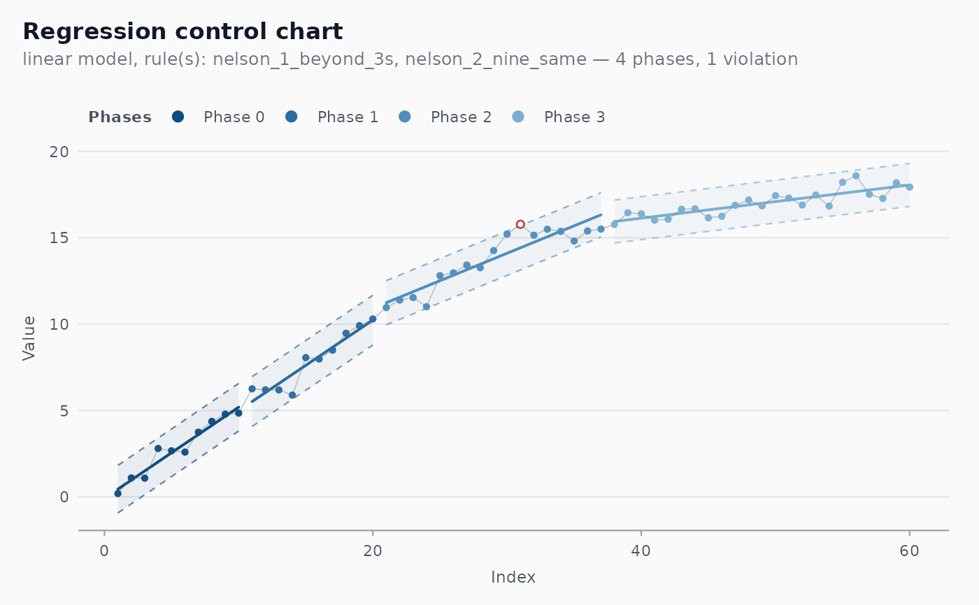
fit <- shewhart_regression(df, value = y, index = t, model = "linear")
print(fit)
#> 
#> ── Shewhart chart regression-based ─────────────────────────────────────────────
#> • Observations / subgroups: 60
#> • Phase: "phase_1"
#> • Sigma estimate ("mr"): 0.4435
#> 
#> ── Control limits ──
#> 
#> # A tibble: 4 × 7
#>   .phase cl_first ucl_first lcl_first cl_last ucl_last lcl_last
#>    <int>    <dbl>     <dbl>     <dbl>   <dbl>    <dbl>    <dbl>
#> 1      0    0.443      1.82    -0.936    5.19     6.57     3.81
#> 2      1    5.52       6.96     4.07    10.2     11.7      8.79
#> 3      2   11.2       12.5      9.96    16.3     17.6     15.0 
#> 4      3   15.9       17.2     14.7     18.1     19.3     16.8 
#> ── Rule violations ──
#> 
#> ! 1 violation across 2 rules.
#> nelson_1_beyond_3s: 1 hit.
ggplot2::autoplot(fit)


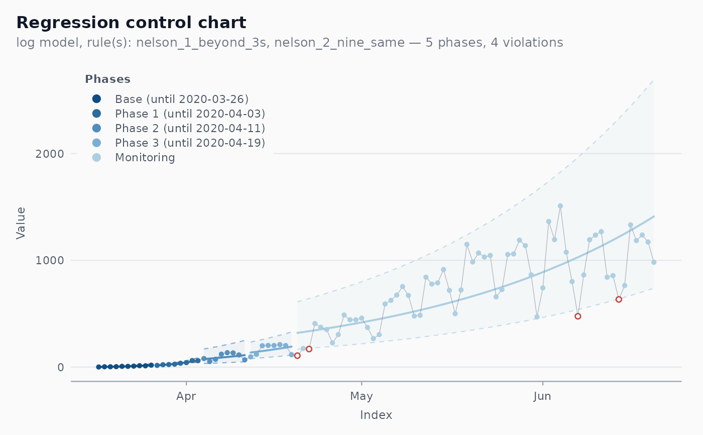
# Multiplicative limits built on the log scale (Perla et al. 2020;
# Ferraz et al. 2020): base of 10 days, 7-point shift rule
br <- subset(cvd_brazil, region == "BR" & date >= as.Date("2020-03-17") &
               date <= as.Date("2020-06-20"))
fit_log <- shewhart_regression(br, value = new_deaths, index = date,
                               model = "log", limits_scale = "model",
                               phase_rule = "we_seven_same")
ggplot2::autoplot(fit_log, legend_position = "inside")

# }