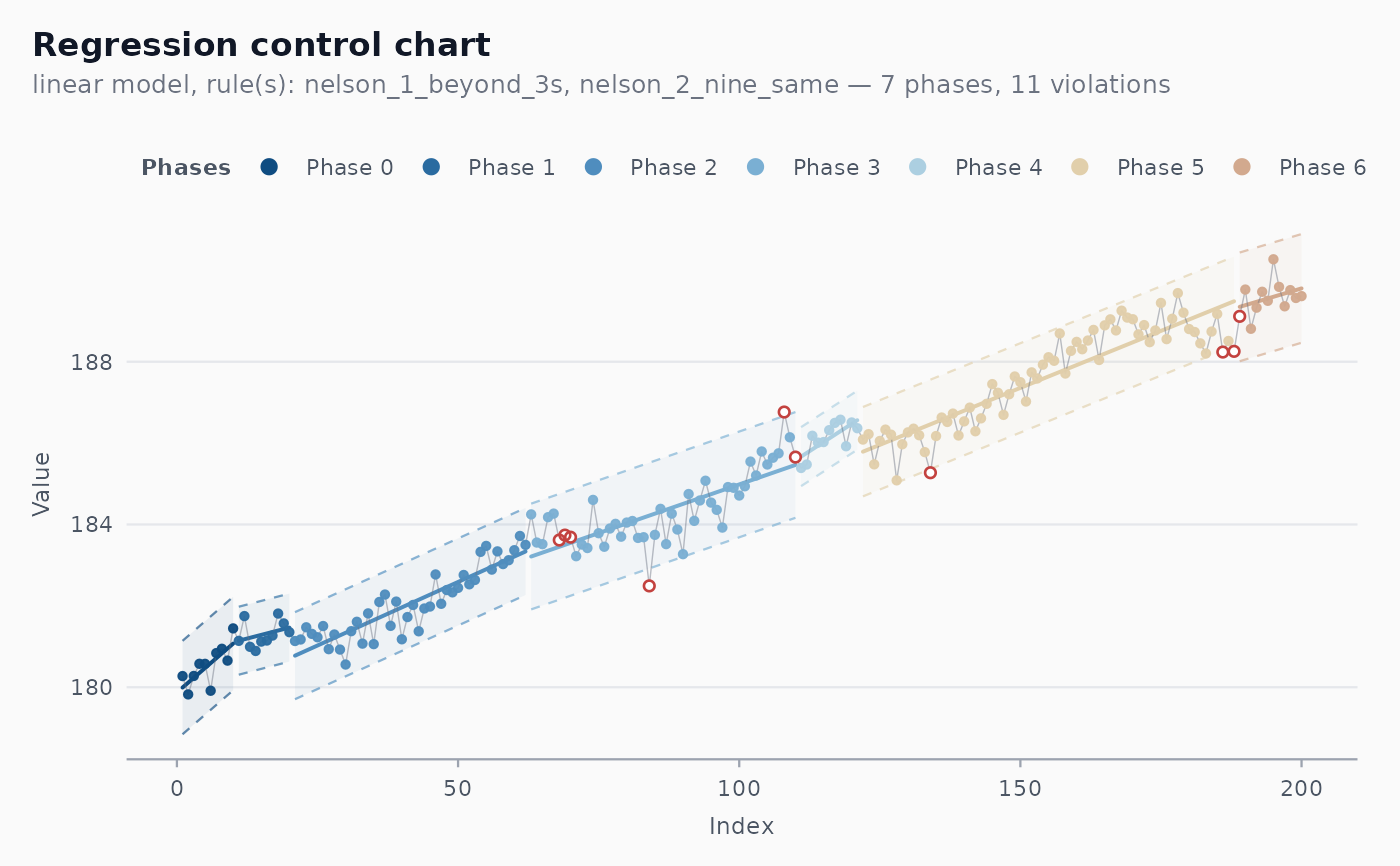
A synthetic dataset of 200 sensor readings on a curing oven. The true temperature exhibits a slow linear drift superimposed on a periodic component. A classical Shewhart chart will misjudge the limits because the process is non-stationary - a regression control chart is the right tool.
Format
A tibble with 200 rows and 2 columns:
- minute
Integer minute since start.
- temp_c
Numeric temperature in degrees Celsius.
Examples
# \donttest{
fit <- shewhart_regression(temperature_drift,
                           value = temp_c, index = minute,
                           model = "linear")
ggplot2::autoplot(fit)

# }
# }